Review of Basic Statistical Concepts

1. Review of Basic Statistical Concepts Farideh Dehkordi-Vakil

2. Review of Basic Statistical Concepts • Descriptive Statistics • Methods that organize and summarize data. • Numerical summary • Graphical Methods • Inferential Statistics • Generalizing from a sample to the population from which it was selected. • Estimation • Hypothesis testing

3. Review of Basic Statistical Concepts • Population • The entire collection of individuals or objects about which information is desired. • Sample • A subset of the population selected in some prescribed manner for study.

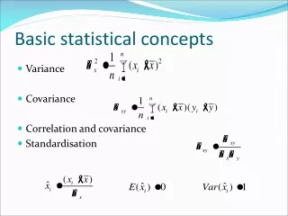
4. Review of Basic Statistical Concepts • Numerical summaries • Measure of central tendencies • Mean • Median • Measure of variability • Variance, Standard deviation • Range • Quartiles

5. Review of Basic Statistical Concepts • The Mean • To find the mean of a set of observations, add their values and divide by the number of observations. If the n observations are , their mean is • In a more compact notation,

6. Example: Books Page Length A sample of n = 8 books is selected from a library’s collection, and page length of each one is determined, resulting in the following data set. X1=247, X2=312, X3=198, X4=780, X5=175, X6=286, X7=293, X8=258

7. Review of Basic Statistical Concepts • Median M • The Median M is the midpoint of a distribution, the number such that half of the observations are smaller and the other half are larger. To find the median of a distribution: • Arrange all observations in order of size, from smallest to largest. • If the number of observations n is odd, the median M is the center observation in the ordered list. • If the number of observations n is even, the median M is the mean of the two center observations in the ordered list.

8. Review of Basic Statistical Concepts • Quartiles Q1 and Q3 • To calculate the quartiles: • Arrange the observations in increasing order and locate the median M in the ordered list of observations. • The first quartile Q1 is the median of the observations whose position in the ordered list is to the left of the location of the overall median. • The third quartile Q3 is the median of the observations whose position in the ordered list is to the right of the location of the overall median.

9. Example: Books Page Length • Median: • Order the list 175, 198, 247, 258, 286, 293, 312, 780 • There are two middle numbers 258, and 286. • The median is the average of these two numbers

10. Review of Basic Statistical Concepts • The Five Number Summary and Box-Plot • The five number summary of a distribution consists of the smallest observation, the first quartile, the median, the third quartile, and the largest observation, written in order from smallest to largest. In symbols, the five number summary is: Minimum Q1 M Q3 Maximum

11. Review of Basic Statistical Concepts • A box-plot is a graph of the five number Summary. • A central box spans the quartiles. • A line in the box marks the median. • Lines extend from the box out to the smallest and largest observations. • Box-plots are most useful for side-by-side comparison of several distributions.

12. Review of Basic Statistical Concepts

13. Review of Basic Statistical Concepts • The Variance s2 • The Variance s2 of a set of observations is the average of the squares of the deviations of the observations from their mean. In symbols, the variance of n observations is • or, more compactly,

14. Review of Basic Statistical Concepts • The Standard Deviation s • The standard deviation s is the square root of the variance s2: • Computational formula for variance

15. Example: Book page length

16. Review of Basic Statistical Concepts • Choosing a Summary • The five number summary is usually better than the mean and standard deviation for describing a skewed distribution or a distribution with extreme outliers. Use , and s only for reasonably symmetric distributions that are free of outliers.

17. Review of Basic Statistical Concepts • Introduction to Inference • The purpose of inference is to draw conclusions from data. • Conclusions take into account the natural variability in the data, therefore formal inference relies on probability to describe chance variation. • We will go over the two most prominent types of formal statistical inference • Confidence Intervals for estimating the value of a population parameter. • Tests of significance which asses the evidence for a claim. • Both types of inference are based on the sampling distribution of statistics.

18. Review of Basic Statistical Concepts • Parameters and Statistics • A parameter is a number that describes the population. • A parameter is a fixed number, but in practice we do not know its value. • A statistic is a number that describes a sample. • The value of a statistic is known when we have taken a sample, but it can change from sample to sample. • We often use statistic to estimate an unknown parameter.

19. Review of Basic Statistical Concepts • Since both methods of formal inference are based on sampling distributions, they require probability model for the data. • The model is most secure and inference is most reliable when the data are produced by a properly randomized design. • When we use statistical inference we assume that the data come from a randomly selected sample (SRS) or a randomized experiment.

20. Example:Consumer attitude towards shopping • A recent survey asked a nationwide random sample of 2500 adults if they agreed or disagreed with the following statement I like buying new cloths, but shopping is often frustrating and time consuming. • Of the respondents, 1650 said they agreed. • The proportion of the sample who agreed that cloths shopping is often frustrating is:

21. Example:Consumer attitude towards shopping • The number = .66 is a statistic. • The corresponding parameter is the proportion (call it P) of all adult U.S. residents who would have said “Yes” if asked the same question. • We don’t know the value of parameterP, so we use as its estimate.

22. Review of Basic Statistical Concepts • If the marketing firm took a second random sample of 2500 adults, the new sample would have different people in it. • It is almost certain that there would not be exactly 1650 positive responses. • That is, the value of will vary from sample to sample. • Random samples eliminate bias from the act of choosing a sample, but they can still be wrong because of the variability that results when we choose at random.

23. ● ● ● ● ● ● ● ● ● ● ● ● ● ● ● ● ● ● ● ● ● ● ● ● ● ● ● ● ● ● ● ● ● ● ● ● ● ● ● ● ● ● ● ● ● ● ● ● ● ● ● ● ● ● ● ● ● ●

24. Review of Basic Statistical Concepts • The first advantage of choosing at random is that it eliminates bias. • The second advantage is that if we take lots of random samples of the same size from the same population, the variation from sample to sample will follow a predictable pattern. • All statistical inference is based on one idea: to see how trustworthy a procedure is, ask what would happen if we repeated it many times.

25. Review of Basic Statistical Concepts • Sampling Distribution of Statistics • Suppose that exactly 60% of adults find shopping for cloths frustrating and time consuming. • That is, the truth about the population is that P = 0.6. (parameter) • We select a SRS (Simple Random Sample) of size 100 from this population and use the sample proportion( , statistic) to estimate the unknown value of the population proportion P. • What is the distribution of ?

26. Review of Basic Statistical Concepts • To answer this question: • Take a large number of samples of size 100 from this population. • Calculate the sample proportion for each sample. • Make a histogram of the values of . • Examine the distribution displayed in the histogram for shape, center, and spread, as well as outliers or other deviations.

27. Review of Basic Statistical Concepts • The result of many SRS have a regular pattern. • Here we draw 1000 SRS of size 100 from the same population. • The histogram shows the distribution of the 1000 sample proportions

28. Review of Basic Statistical Concepts • Sampling Distribution • The sampling distribution of a statistic is the distribution of values taken by the statistic in all possible samples of the same size from the same population.

29. Normal Distribution • These curves, called normal curves, are • Symmetric • Single peaked • Bell shaped • Normal curves describe normal distributions.

30. Normal Density Curve • The exact density curve for a particular normal distribution is described by giving its mean  and its standard deviation . • The mean is located at the center of the symmetric curve and it is the same as the median. • The standard deviation  controls the spread of a normal curve.

31. Normal Density Curve

32. Standard Normal Distribution • The standard Normal distribution is the Normal distribution N(0, 1) with mean  = 0 and standard deviation  =1.

33. Standard Normal Distribution • If a variable x has any normal distribution N(, ) with mean  and standard deviation , then the standardized variable has the standard Normal distribution.

34. The Standard Normal Table • Table A is a table of the area under the standard Normal curve. The table entry for each value z is the area under the curve to the left of z.

35. The Standard Normal Applet • Or you can use this applet http:/www.stat.sc.edu~west/applets/normaldemo.html

36. The Standard Normal Table • What is the area under the standard normal curve to the right of z = - 2.15? • Compact notation: • P = 1 - .0158 =.9842

37. The Standard Normal Table • What is the area under the standard normal curve between z = 0 and z = 2.3? • Compact notation: • P = .9893 - .5 =.4893

38. Example:Annual rate of return on stock indexes The annual rate of return on stock indexes (which combine many individual stocks) is approximately Normal. Since 1954, the Standard & Poor’s 500 stock index has had a mean yearly return of about 12%, with standard deviation of 16.5%. Take this Normal distribution to be the distribution of yearly returns over a long period. The market is down for the year if the return on the index is less than zero. In what proportion of years is the market down?

39. Example:Annual rate of return on stock indexes • State the problem • Call the annual rate of return for Standard & Poor’s 500-stocks Index x. The variable x has the N(12, 16.5) distribution. We want the proportion of years with X < 0. • Standardize • Subtract the mean, then divide by the standard deviation, to turn x into a standard Normal z:

40. Example:Annual rate of return on stock indexes • Draw a picture to show the standard normal curve with the area of interest shaded. • Use the table • The proportion of observations less than - 0.73 is .2327. • The market is down on an annual basis about 23.27% of the time.

41. Example:Annual rate of return on stock indexes • What percent of years have annual return between 12% and 50%? • State the problem • Standardize

42. Example:Annual rate of return on stock indexes • Draw a picture. • Use table. • The area between 0 and 2.30 is the area below 2.30 minus the area below 0. 0.9893- .50 = .4893

43. Estimation • So far, we have used our sample estimates as point estimates of parameters, for example: • These estimators have properties.

44. Estimators • They are both unbiased estimators • The expected value of an unbiased estimator is equal to the parameter that it is trying to estimate.

45. Estimators • For Example: • It tends to give an answer that is a little too small.

46. Estimators • is also a minimum variance estimator of . • This means that it has the smallest variability among all estimators of . • What if we want to do more than just provide a point estimate?

47. Estimating with Confidence • Suppose we are interested in the value of some parameter, and we want to construct a confidence interval for it, with some desired level of confidence

48. Estimating with Confidence • Suppose we can estimate this parameter from sample data, and we know the distribution of this estimator, then we can use this knowledge and construct a probability statement involving both the estimator and the true value of the parameter. • This statement is manipulated mathematically to produce confidence intervals.

49. Confidence intervals • The general form of a confidence interval is: sample value of estimator  (Factor)(SE of estimator) • The value of the factor will depend on the level of confidence desired, and the distribution of the estimator.

50. Estimating with Confidence • Community banks are banks with less than a billion dollars of assets. There are approximately 7500 such banks in the United States. In many studies of the industry these banks are considered separately from banks that have more than a billion dollars of assets. The latter banks are called “large institutions.” The community bankers Council of the American bankers Association (ABA) conducts an annual survey of community banks. For the 110 banks that make up the sample in a recent survey, the mean assets are = 220 (in millions of dollars). What can we say about , the mean assets of all community banks?