Production Plant Layout (1)
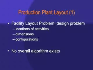
Production Plant Layout (1). Facility Layout Problem: design problem locations of activities dimensions configurations No overall algorithm exists. Design problem. Greenfield. Location of one new machine. Production Plant Layout (2). Production Plant Layout (2). Reasons: new products

Production Plant Layout (1)
E N D
Presentation Transcript
Production Plant Layout (1) • Facility Layout Problem: design problem • locations of activities • dimensions • configurations • No overall algorithm exists
Design problem Greenfield Location of one new machine Production Plant Layout (2) Production Plant Layout (2) • Reasons: • new products • changes in demand • changes in product design • new machines • bottlenecks • too large buffers • too long transfer times
Product Layout Logistics Process Design
Production Plant Layout (3) • Goals (examples): • minimal material handling costs • minimal investments • minimal throughput time • flexibility • efficient use of space
Production Plant Layout (4) • Restrictions: • legislation on employees working conditions • present building (columns/waterworks) • Methods: • Immer: The right equipment at the right place to permit effective processing • Apple: Short distances and short times
Goals Production Plant Layout • Plan for the preferred situation in the future • Layout must support objectives of the facility • No accurate data layout must be flexible
1 Flow 2 Activities Analysis 3 Relationship diagram 4 Space requirements 5 Space available 6 Space relationship diagram Search 7 Reasons to modify 8 Restrictions 9 Layout alternatives Selection 10 Evaluation Systematic Layout Planning Muther (1961) 0 Data gathering
product design sequence of assembly operations machines layout (assembly) line 0 - Data gathering (1) • Source: product design • BOM • drawings • “gozinto” (assembly) chart, see fig 2.10 • redesign, standardization simplifications
0 - Data gathering (2) • Source: Process design • make/buy • equipment used • process times operations process chart (fig 2.12) assembly chart operations precedence diagram (fig 2.13)
0 - Data gathering (3) • Source: Production schedule design • logistics: where to produce, how much product mix • marketing: demand forecast production rate • types and number of machines • continuous/intermittent • layout schedule
1/2 - Flow and Activity Analysis • Flow analysis: • Types of flow patterns • Types of layout flow analysis approaches • Activity relationship analysis
1/2 - Flow analysis and activity analysis Flow analysis • quantitative measure of movements between departments:material handling costs Activity analysis • qualitative factors
Raw material Finished product Flow analysis • Flow of materials, equipment and personnel layout facilitates this flow
R S R S S long line R Types of flow patterns • Horizontal transport P = receiving S = shipping
Layout volumes of production variety of products • volumes: what is the right measure of volume from a layout perspective? • variety high/low commonality layout type
Types of layout • Fixed product layout • Product layout • Group layout • Process layout
Fixed product layout • Processes product (e.g. shipbuilding)
Product layout (flow shop) • Production line according to the processing sequence of the product • High volume production • Short distances
Process layout (Job shop) • All machines performing a particular process are grouped together in a processing department • Low production volumes • Rapid changes in the product mix • High interdepartmental flow
Group layout • Compromise between product layout and process layout • Product layouts for product families cells (cellular layout) • Group technology
product layout group layout process layout production volume product variety Production volume and product variety determines type of layout
Layout determines • material handling • utilization of space, equipment and personnel (table 2.2) Flow analysis techniques • Flow process charts product layout • From-to-chart process layouts
Activity relationship analysis • Relationship chart (figure 2.24) • Qualitative factors (subjective!) • Closeness rating (A, E, I, O, U or X)
3 - Relationship diagrams • Construction of relationships diagrams: diagramming • Methods, amongst others: CORELAP
Relationship diagram (1) • Spatial picture of the relationships between departments • Constructing a relation diagram often requires compromises. What is closeness? 10 or 50 meters? • See figure 2.25
Relationship diagram (2) Premise: geographic proximity reflects the relationships Sometimes other solutions: • e.g. X-rating because of noise acoustical panels instead of distance separation • e.g. A rating because of communication requirement computer network instead of proximity
Graph theory based approach • close adjacent • department-node • adjacent-edge • requirement: graph is planar (no intersections) • region-face • adjacent faces: share a common edge graph
Primal graph dual graph • Place a node in each face • Two faces which share an edge – join the dual nodes by an edge • Faces dual graph correspond to the departments in primal graph block layout (plan) e.g. figure 2.39
Graph theory • Primal graph planar dual graph planar • Limitations to the use of graph theory: it may be an aid to the layout designer
CORELAP • Construction “algorithm” • Adjacency! • Total closeness rating = sum of absolute values for the relationships with a particular department.
CORELAP - steps • sequence of placements of departments • location of departments
CORELAP – step 1 • First department: • Second department: • X-relation “last placed department” • A-relation with first. If none E-relation with first, etcetera
2 3 4 8 1 7 6 5 2nd 1st CORELAP – step 2 • Weighted placement value
4 - Space requirements • Building geometry or building site space available • Desired production rate, distinguish: • Engineer to order (ETO) • Production to order (PTO) • Production to stock (PTS) marketing forecast productions quantities
rate machine operators machines employees assembly 4 - Space requirements Equipment requirements: • Production rate number of machines required • Employee requirements
Space determination Methods: 1. Production center 2. Converting 4. Standards 5. Projection
# machines per operator # assembly operators Space requirements 4 - Space determination (1) 1. Production center • for manufacturing areas • machinespace requirements 2. Converting • e.g. for storage areas • present space requirement space requirements • non-linear function of production quantitiy
4 - Space determination (2) • Space standards • standards • Ratio trend and projection • e.g. direct labour hour, unit produced • Not accurate! • Include space for: packaging, storage, maintenance, offices, aisles, inspection, receiving and shipping, canteen, tool rooms, lavatories, offices, parking
Deterministic approach (1) • n’ = # machines per operator (non-integer) • a = concurrent activity time • t = machine activity time • b= operator
Deterministic approach (2) • Tc = cycle time • a = concurrent activity time • t = machine activity time • b = operator activity time • m = # machines per operator
Deterministic approach (3) • TC(m) = cost per unit produced as a function of m • C1 = cost per operator-hour • C2 = cost per machine-hour • Compare TC(n) and TC(n+1) for n < n’ < n+1
Designing the layout (1) • Search phase • Alternative layouts • Design process includes • Space relationship diagram • Block plan • Detailed layout • Flexible layouts • Material handling system • Presentation
Designing the layout (2) • Relationship diagram + space space relationship diagram (see fig 2.56) • Different shapes
selection detailed design detailed design selection or 9 – Layout alternatives • Alternative layouts by shifting the departments to other locations block plan, also shows e.g. columns and positions of machines (see fig 2.57)
Flexible layouts • Future • Anticipate changes • 2 types of expansion: • sizes • number of activities
Material handling system • Design in parallel with layout • Presentation • CAD templates 2 or 3 dimensional • simulations • “selling” the layout (+ evaluation)
10 Evalution (1) Selection and implementation • best layout • cost of installation + operating cost • compare future costs for both the new and the old layout • other considerations • selling the layout • assess and reduce resistance • anticipate amount of resistance for each alternative
10 Evalution (2) • Causes of resistance: • inertia • uncertainty • loss of job content • … • Minimize resistance by • participation • stages
Implementation • Installation • planning • Periodic checks after installation
0 Data gathering 1 Flow 2 Activities Analysis 3 Relationship diagram 4 Space requirements 5 Space available 6 Space relationship diagram Search 7 Reasons to modify 8 Restrictions 9 Layout alternatives Selection 10 Evaluation Systematic Layout Planning