Simulink Stability Analysis
Computing Steady-State Solutions. Matlab function trim ? finds steady state solutions for a Simulink system >> [x,u,y,dx]=trim(sys,x0,x0)Attempts to find values for x, u and y that set the state derivatives, dx, of the S-function sys to zero using a constrained optimization technique.Sets the ini


Simulink Stability Analysis
E N D
Presentation Transcript
1. Simulink Stability Analysis Computing steady-state solutions
Constructing linearized models
Biochemical reactor example
2. Computing Steady-State Solutions Matlab function trim � finds steady state solutions for a Simulink system
>> [x,u,y,dx]=trim(sys,x0,x0)
Attempts to find values for x, u and y that set the state derivatives, dx, of the S-function sys to zero using a constrained optimization technique.
Sets the initial starting guesses for x and u to x0 and u0, respectively.
3. Computing Linearized Models Matlab function linearize � obtains a linear model from a Simulink model
>> linsys = linearize(sys,sys_io)
Takes a Simulink model, sys, and an I/O object, sys_io, as inputs and returns a linear state-space model, linsys. The linearization I/O object is created with the function linio.
>> sys_io=linio(blockname,portnum,type)
Creates a linearization I/O object for the signal that originates from the outport with port number, portnum, of the type given by type of the block, blockname, in a Simulink model. Available linearization I/O types include:
'in', linearization input point
'out', linearization output point
4. Biochemical Reactor Example Continuous bioreactor model
Parameter values
KS = 1.2 g/L, mmax = 0.48 h-1, YX/S = 0.4 g/g
D = 0.15 h-1, Si = 20 g/L
Steady-state solutions
Eigenvalues
5. Simulink Model
6. S-Function
7. S-Function cont.
8. S-Function cont.
9. In-Class Exercise Use the Matlab function trim to find the two steady-state solutions
Use the Matlab function linearize to find a linear model at the non-trivial steady state
Use the Matlab function eig to check the stability of the non-trivial steady state
10. Steady-State Solutions >> sys = 'bioreactor_stability';
>> load_system(sys);
>> open_system(sys);
>> [x1,u1,y1,dx1]=trim(sys,[1; 1],[]);
>> x1
x1 =
7.7818
0.5455
>> [x2,u2,y2,dx2]=trim(sys,[0; 0],[]);
>> x2
x2 =
0.0000
20.0000
11. Linear Model Analysis >> sys_io(1)=linio('bioreactor_stability/Dilution',1,'in');
>> sys_io(2)=linio('bioreactor_stability/Bioreactor',1,'out');
>> linsys = linearize(sys,sys_io)
a =
Bioreactor(1 Bioreactor(2
Bioreactor(1 -8.596e-005 1.472
Bioreactor(2 -0.3748 -3.829
b =
Dilution (pt
Bioreactor(1 -7.78
Bioreactor(2 19.45
c =
Bioreactor(1 Bioreactor(2
bioreactor_s 1 0
d =
Dilution (pt
bioreactor_s 0
>> lambda=eig(linsys.a)
lambda =
-0.1500
-3.6793