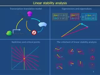
Local Stability Analysis

1. Local Stability Analysis Step One: find stationary point(s) Step Two: linearize around all stationary points (using Taylor expansion), the Eigenvalues of the linearized problem determine nature of stationary point: Real parts: positive: growth of fluctuations, instability negative: decay of fluctuations, stability Imaginary parts: if present, solutions are oscillatory (spiraling) spiraling inward or outward if non-zero real parts Overall: point (asymptotically) stable if all real parts negative

2. a. b. c. Examples of nonlinear activation functions (transfer functions): a. “half-wave rectification” b. “sigmoidal function” Note: we will typically consider the activation function as a fixed property of our model neurons but real neurons can change their intrinsic properties. c. rectified hyperbolic tangent

3. The Naka-Rushton function A good fit for the steady state firing rate of neurons in several visual areas (LGN, V1, middle temporal) in response to a visual stimulus of contrast P is given by: P ½ , the “semi-saturation”, is the stimulus contrast (intensity) that produces half of the maximum firing rate rmax. N determines the slope of the non-linearity at P ½ . Albrecht and Hamilton (1982)

4. Interaction of Excitatory and Inhibitory Neuronal Populations • Motivations: • understand the emergence of oscillations in excitatory-inhibitory networks • learn about local stability analysis • Consider 2 populations of excitatory and inhibitory neurons with firing rates v: MIE MEE vE vI MEI Dale’s law: every neuron is either excitatory or inhibitory, never both

5. vE vI MIE MEE MEI Mathematical formulation: [ ]+ Parameters: MEE= 1.25, MEI = -1, gammaE = -10Hz, tauE = 10ms MII= 0, MIE = 1, gammaI = 10 Hz, tauI = varying Stationary point:

6. Phase Portrait *nullclines, zero-isoclines stationary point * * A: Stationary point is intersection of the nullclines. Arrows indicate direction of flow in different area of the phase space (state space). B: real and imaginary part of Eigenvalue as a function of tauI .

7. Linearization around stationary point gives the following matrix A with these Eigenvalues:

8. For tauI below critical value of 40ms, Eigenvalues have negative real parts: we see damped oscillations. Trajectory spirals to stable fixed point

9. When tauI grows beyond critical value of 40ms, a Hopf bifurcation occurs (here tauI=50ms): stable fixed point → unstable fixed point + limit cycle Here, the amplitude of the oscillation grows until the non-linearity “clips” it.

10. Neural Oscillations • interaction of excitatory and inhibitory neuron populations can lead to oscillations • very important in, e.g. locomotion: rhythmic walking and swimming motions: Central Pattern Generators (CPGs) • also very important in olfactory system (selective amplification) • also oscillations in visual system: functional role hotly debated. Proposed as solution to binding problem: • Idea: neural populations that represent features of the same object synchronize their firing

11. Binding Problem • what and where (how) pathways in visual system • how do you know what is where? Synchronization no yes circle triangle up visual field down neural representation spike trains

12. K1 K2 Competition and Decisions Motivation:ability to decide between alternatives is fundamental Idea: inhibitory interaction between neuronal populations representing different alternatives is plausible candidate mechanism The most simple system: Winner-take-all (WTA) network

13. Stationary States and Stability • The stationary states for K1=K2=120: • e1 = 50, e2 = 0 • e2 = 50, e1 = 0 • e1 = e2 = 20 Linear stability analysis: 1) for e1 = 50, e2 = 0 : 2) for e1 = e2 = 20 : (τ=20ms) → “stable node” → “unstable saddle”

14. Matlab Simulation Behavior for strong identical input: K1=K2=K=120 one unit wins the competition and completely suppresses the other

15. Continuous Neural Fields So far: individual units, with specific connectivity patterns Idea: abstract from individual neurons to continuous fields of neurons, where synaptic weights patterns become homogeneous interaction kernels Variant 1: continuous labeling of input or output domain Variant 2: continuous labeling of two-dimensional cortical space

16. Recurrent Simple Cell Model Question:how is orientation selectivity achieved? (feedforward vs. recurrent accounts)

17. Classic Hubel and Wiesel Model complex cell sums inputs from simple cells with same orientation but different phase preference simple cell sums input from geniculate On and Off cells in particular constellation

18. Recurrent Model Stimulus with orientation angle θ=0. A: amplitude, c: contrast, ε: small nonlinear amplification

19. Superior Colliculus and Saccades Representation of saccade motor command in superior colliculus: vector averaging Yarbus

20. A Simple Model of Saccade Target Selection Question:how do you select the target of your next saccade? Idea: competitive “blob” dynamics in 2 dimensional “neural field” linear unit for global inhibition layer of non-linear units with local excitation

21. Reminder: Convolution Stability Analysis of Saccade Model Step 1:look for homogeneous stationary solutions Step 2: find range of β for which homogeneous stationary solution becomes unstable Step 3: simulate system (Matlab), observe behavior Step 4: estimate the size of the resulting blob as a function of β

22. Example Run Initialization:10 random spots of small activity, I=0, η small Gaussian iid noise time Result:a blob of activity forms at location determined by initial state and noise

23. Results of Analysis • Step 1:look for homogeneous stationary solutions • h0=0 works, β>1/A prevents fully active layer (A=area of layer) • Step 2: find range of β for which homogeneous stationary solution becomes unstable • for small local fluctuation from h0=0 to grow, we need β<1/2πσ2 • Step 3: simulate system (Matlab), observe behavior • formation of single blob of activity suppressing all other activity in layer • Step 4: estimate the size of the resulting blob as a function of β, σ

24. Matlab Code Fragments % initialize layer size = 50; h = zeros(size,size); for i=1:10 x = unidrnd(size); y = unidrnd(size); h(x,y)=h(x,y)+0.05; end % main loop while(1) active = (h>0); I = conv2(active, g, 'same') - beta*(sum(sum(active))); h = (1-alpha)*h + alpha*I + normrnd(0, noise, size, size); % display plots, etc. pause end

25. Discussion of Saccade Model • Positive: • roughly consistent with anatomy/physiology • explains how several close-by targets can win over strong but isolated target • suggests why time to decision is longer in situations with several equally strong targets • similar models used in modeling human performance in visual search tasks • Limitations: • only qualitative account • in order to make precise quantitative predictions, it is typically necessary to take more physiological details into account, which are mostly unknown: • exact connectivity patterns • non-linearities • more than one area is involved • what are all the inputs?

26. Population vector decoding: where ca is the preferred stimulus vector for unit a Connection to Maximum Likelihood Estimation So far: purely bottom-up view: networks with this connectivity structure just happen to exhibit this behavior and this may be analogous to what the brain does New idea: use such dynamics to do Maximum Likelihood estimation Want: New idea: blob dynamics + vector decoding works better than doing direct vector decoding on the noisy inputs r: firing rate vector, Θ: stimulus parameter 1-d “blob” network with noisy input

27. Binocular Rivalry, Bistable Percepts Idea: extend WTA network by slow adaptation mechanism. Adaptation acts to increase semi-saturation of Naka Rushton non-linearity ambiguous figure binocular rivalry L R

28. Matlab Simulation β=1.5 β=1.5

29. Discussion of Rivalry Model • Positive: • roughly consistent with anatomy/physiology • offers parsimonious mechanism for different perceptual switching phenomena, in a sense it “unifies” different phenomena by explaining them with the same mechanism • Limitations: • provides only qualitative account • real switching behaviors are not so nice and regular and simple: • cycles of different durations • temporal asymmetries • rivalry: competition likely takes place in hierarchical network rather than in just one stage. • spatial dimension was ignored