Summary of full OSSEs at NCEP and Emerging Internationally Collaborative Joint OSSEs

1. Summary of full OSSEs at NCEP and Emerging Internationally Collaborative Joint OSSEs Joint OSSE Team http://www.emc.ncep.noaa.gov/research/JointOSSEs http://www.emc.ncep.noaa.gov/research/THORPEX/osse

2. Speakers Introduction to OSSEs and Summary of NCEP Michiko Masutani (EMC) Introduction to Joint OSSEs and Joint OSSE NR Michiko Masutani (EMC), Erik Andersson (ECMWF) Evaluation of Joint OSSE Nature Run Oreste Reale (NASA/GSFC), Erik Andersson (ECMWF) Strategies of Simulation of Observation Jack Woollen (EMC) Simulation of Dopler Wind Lidar (DWL) Dave Emmitt(Simpson Weather Associates) Progress and Plans in Joint OSSE Michiko Masutani (EMC) OSSEs in the Joint Center for Satellite Data Assimilation Lars Peter Riishojgaard (Director of Joint Center for Satellite Data Assimilation)

3. Introduction to OSSE and Summary of NCEP OSSEs Michiko Masutani NOAA/NWS/NCEP/EMC RSIS/Wyle Information Systems http://www.emc.ncep.noaa.gov/research/OSSE

4. Co-Authors and Contributors to NCEP OSSEs Michiko Masutani, John S. Woollen, Stephen J. Lord, Yucheng Song, Zoltan Toth,Russ Treadon NCEP/EMC Haibing Sun, Thomas J. Kleespies NOAA/NESDIS G. David Emmitt , Sidney A. Wood, Steven Greco Simpson Weather Associates Joseph Terry NASA/GSFC Acknowledgement: John C. Derber, Weiyu Yang, Bert Katz, Genia Brin, Steve Bloom, Bob Atlas, V. Kapoor, Po Li, Walter Wolf, Jim Yoe, Bob Kistler, Wayman Baker, Tony Hollingsworth, Roger Saunder, and many moor

5. Nature Run Nature Run Nature Run: Serves as a true atmosphere for OSSEs Observational data will be simulated from the Nature Run

6. Nature Run Existing data + Proposed data DWL, CrIS, ATMS, UAS, etc Current observing system DATA PRESENTATION OSSE DATA PRESENTATION OSSE Quality Control (Simulated conventional data) Real TOVS AIRS etc. Quality Control (Real conventional data) Simulated TOVS AIRS etc. OSSE DA DA OSSE GFS NWP forecast NWP forecast

7. Need for OSSEs ♦Quantitatively–based decisions on the design and implementation of future observing systems ♦ Evaluate possible future instruments without the cost of developing, maintaining & using observing systems. Benefit of OSSEs ●OSSEs help understanding and formulation of observational errors ●DA (Data Assimilation) system will be prepared for the new data ●Enable data formatting and handling in advance of “live” instrument ● The OSSE results also showed that theoretical explanations will not be satisfactory when designing future observing systems.

8. Full OSSE There are many types of simulation experiments. We have to call our OSSE as Full OSSE to avoid confusion. ●Nature run (proxy true atmosphere) is produced from a free forecast run using the highest resolution operational model. ●Calibration to compare data impact between real and simulated data impact will be performed. ●Data impact on forecast will be evaluated ●Full OSSE can provide detail evaluation about configuration of observing systems.

9. Summary of results from NCEP OSSE • Winter time Nature run (1 month, Feb5-Mar.7,1993) • NR by ECMWF model T213 (~0.5 deg) • 1993 data distribution for calibration • NCEP DA (SSI) withT62 ~ 2.5 deg, 300km and T170 ~1 deg, 110km • Simulate and assimilate level1B radiance • Different method than using interpolated temperature as retrieval • Use line-of- sight (LOS) wind for DWL • not u and v component • Calibration performed • Effects of observational error tested • NR clouds are evaluated and adjusted at NCEP

10. Compare real data sensitivity to sensitivity with simulated data Impact of withdrawing RAOB winds OSSE Calibration

11. Results from OSSEs forDoppler Wind Lidar (DWL) All levels (Best-DWL): Ultimate DWL that provides full tropospheric LOS soundings, clouds permitting. DWL-Upper: An instrument that provides mid and upper tropospheric winds only down to the levels of significant cloud coverage. DWL-PBL: An instrument that provides only wind observations from clouds and the PBL. Non-Scan DWL : A non-scanning instrument that provides full tropospheric LOS soundings, clouds permitting, along a single line that parallels the ground track. (ADM-Aeolus like DWL) Zonally and time averaged number of DWL measurements in 2.5 degree grid box with 50km thickness in 6 hours. Numbers are devided by 1000. Note that size of 2.5 degree boxes are smaller in higher latitude. Estimate impact of real DWL from combination.

12. Atmospheric Dynamics Mission ADM-Aeolus ADM-Aeolus with single payload Atmospheric LAser Doppler INstrument ALADIN • Observations of Line-of-Sight LOS wind profiles in troposphere to lower stratosphere up to 30 km with vertical resolution from 250 m - 2 km horizontally averaged over 50 km every 200 km • Vertical sampling with 25 range gates can be varied up to 8 times during one orbit • High requirement on random error of HLOS <1 m/s (z=0-2 km, for Δz=0.5 km) <2 m/s (z=2-16 km, for Δz= 1 km), unknown bias <0.4 m/s and linearity error <0.7 % of actual wind speed; HLOS: projection on horizontal of LOS => LOS accuracy = 0.6*HLOS • Operating @ 355 nm with spectrometers for molecular Rayleigh and aerosol/cloud Mie backscatter • First wind lidar and first High Spectral Resolution Lidar HSRL in space to obtain aerosol/cloud optical properties (backscatter and extinction coefficients)

13. Synoptic Scale Total scale 200 mb V 850 mb V Doppler Wind Lidar (DWL) Impactwithout TOVS (using 1999 DAS) Scan_DWL 3 3 Scan_DWL Uniformly thinned to 5% Scan_DWL_upper Scan_DWL_Lower Non_scan_DWL 8 8 No Lidar (Conventional + NOAA11 and NOAA12 TOVS) Time averaged anomaly correlations between forecast and NR for meridional wind (V) fields at 200 hPa and 850 hPa. Experiments are done with 1999 DAS. CTL is assimilation with conventional data only

14. Synoptic Scale Total scale 850 mb V 200 mb V Doppler Wind Lidar (DWL) ImpactWith TOVS (using 2004 DAS) Scan_DWL 1.2 1.2 Scan_DWL Uniformly thinned to 5% Scan_DWL_upper Scan_DWL_Lower 3 3 Non_scan_DWL No Lidar (Conventional + NOAA11 and NOAA12 TOVS) Forecast hour Dashed green line is for scan DWL with 20 time less data to make observation counts similar to non scan DWL. This experiments is done with 2004 DAS.

15. Differences in anomaly correlation Synoptic Scale Total scale 2004 DAS CTL (Conventional + TOVS) 200 mb V - 1999 DAS CTL - CTL (99) - CTL(99) 1999DAS CTL - CTL(99) Data Impact of scan DWL1999 DAS vs. 2004 DAS Impact of 2004 DAS Scan_DWL with 2004 DAS Scan_DWL with 1999 DAS Impact of DWL + better DAS Impact of DWL

16. Differences in anomaly correlation Synoptic Scale Total scale T62 CTL (reference) (Conventional data only) 200 mb V - CTL(T62) - CTL(T62) T170 CTL - CTL (T62) ◊ CTL X CTL+BestDWL Data Impact of scan DWL vs. T170 Impact of DWL + T170 Impact of T170 model Impact of DWL T62 CTL with Scan DWL T170 CTL with Scan DWL In planetary scale increasing morel resolution is more important than adding DWL with scan In smaller scale, adding DWL with scan is more important than increasing model resolution

17. Effect of Observational Error on DWL Impact • Percent improvement over Control Forecast (without DWL) • Open circles: RAOBs simulated with systematic representation error • Closed circles: RAOBs simulated with random error • Green: Best DWL • Blue: Non- Scan DWL 3 3 8 8 Time averaged anomaly correlations between forecast and NR for meridional wind (V) fields at 200 hPa and 850 hPa. Experiments are done with 1999 DAS. CTL is assimilation with conventional data only.

18. DWL-Upper:An instrument that provides mid and upper tropospheric winds only to the levels of significant cloud coverage. Operates only 10% (possibly up to 20%) of the time. Switch on for 10 min at a time. DWL-Lower:An instrument that provides wind observations only from clouds and the PBL. Operates 100% of the time and keeps the instruments warm as well as measuring low level wind DWL-NonScan: DWL covers all levels without scanning (ADM mission type DWL) Targeted DWL experiments(Technologically possible scenarios) Combination of two lidar

19. 200mb (Feb13 - Mar 6 average ) 10% Upper Level Adaptive sampling (based on the difference between first guess and NR, three minutes of segments are chosen – the other 81 min discarded) Doubled contour 100% Upper Level 10% Uniform DWL Upper NonScan DWL

20. 100% Lower + 100% Upper 100% Lower + 10% Targeted Upper 100% Lower + Non Scan 100% Lower + 10% Uniform Upper 100% Lower Non Scan only No Lidar (Conventional + NOAA11 and NOAA12 TOVS) Anomaly correlation difference from control Synoptic scale Meridional wind (V) 200hpa NH Feb13-Feb28 DWL-Lower is better than DWL-NonScan only With 100% DWL-Lower DWL-NonScan is better than uniform 10% DWL-Upper Targeted 10% DWL-Upper performs somewhat better than DWL-NonScan in the analysis DWL-NonScanperforms somewhat better than Targeted 10% DWL-Upperin 36-48 hour forecast CTL

21. Data and model resolution OSSEs with Uniform Data More data or a better model? Fibonacci Grid used in the uniform data coverage OSSE • 40 levels equally-spaced data • 100km, 500km, 200km are tested Skill is presented as Anomaly Correlation % The differences from selected CTL are presented - Yucheng Song Time averaged from Feb13-Feb28 12-hour sampling 200mb U and 200mb T are presented

22. U 200 hPa Benefit from increasing the number of levels 5 500km Raob T62L64 anal T62L64 fcst L64 anl&fcst 500km Raob T62L64 anal T62L28 fcst 500km RaobT62L28 anal & fcst L64 anl L28 fcst 1000km RaobT170L42 analT62L28 fcst CTL 1000km RaobT62L28 anal & fcst T 200 hPa L64 anl&fcst 500km obs T170 L42 model High density observation give better analysis but it could cause poor forecast High density observations give a better analysis but could cause a poor forecast Increasing the vertical resolution was important for high density observations L64 anl L28 fcst

23. Summary The current NCEP OSSEs have demonstrated that OSSEs can provide critical information for assessing observational data impacts. The results also showed that theoretical explanations will not be satisfactory when designing future observing systems. We also experience that conducting reliable OSSEs are much more work than expected. The nature run used was too short and T213 was too cause to continue OSSEs.

24. Introduction to Joint OSSEs and Joint OSSE Nature Runs Michiko Masutani NOAA/NWS/NCEP/EMC Erik Andersson ECMWF http://www.emc.ncep.noaa.gov/research/JointOSSEs

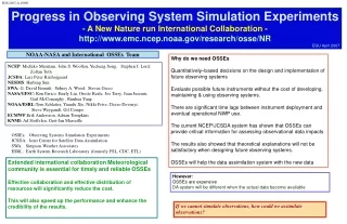
25. Need for collaboration Need one good new Nature Run which will be used by many OSSEs including regional data assimilation. Share the simulated data to compare the OSSE results by various DA systems to gain confidence in results. OSSEs require many experts and requires wide range of resources Extensive international collaboration within the Meteorological community is essential for timely and reliable OSSEs to influence decisions.

26. Joint OSSEs Team Beginning to receive funds but mostly volunteers NCEP: Michiko Masutani, John S. Woollen, Yucheng Song, Stephen J. Lord, Zoltan Toth JCSDA: Lars Peter Riishojgaard (NASA/GFSC), Fuzhong Weng (NESDIS) NESDIS: Haibing Sun, Tong Zhu SWA: G. David Emmitt, Sidney A. Wood, Steven Greco NASA/GFSC: Ron Errico, Oreste Reale, Runhua Yang, Harpar Pryor, Alindo Da Silva, Matt McGill, Juan Juseum, Emily Liu, NOAA/ESRL:Tom Schlatter, Yuanfu Xie, Nikki Prive, Dezso Devenyi, Steve Weygandt ECMWF: Erik Andersson KNMI: Ad Stoffelen, Gert-Jan Marseille MSU/GRI: Valentine Anantharaj, Chris Hill, Pat Fitzpatrick, More people are getting involved or considering perticipation. T. Miyoshi(JMA), Z. Pu(Univ. Utah), Lidia Cucil (EMC, JCSDA), G. Compo(ESRL), Prashant D Sardeshmukh(ESRL), M.-J. Kim(NESDIS), T. Enomoto(JEMSTEC), Jean Pailleux(Meteo France), Roger Saunders(Met Office), C. O’Handley(SWA), E Kalnay(U.MD), A.Huang (U. Wisc), Craig Bishop(NRL) People who helped or advised Joint OSSEs Joe Terry, K. Fielding (ECMWF), S. Worley (NCAR), C.-F., Shih (NCAR), Y. Sato (NCEP,JMA), M. Yamaguchi (JMA), Lee Cohen(ESRL), David Groff(NCEP), Daryl Kleist(NCEP), J Purser(NCEP), Bob Atlas(NOAA/AOML),M.Hart(EMC), C. Sun (BOM), M. Hart(NCEP), G. Gayno(NCEP), W. Ebisuzaki (NCEP), A. Thompkins (ECMWF), S. Boukabara(NESDIS), John Derber(NCEp), X. Su (NCEP), R. Treadon(NCEP), P. VanDelst (NCEP), M Liu(NESDIS), Y Han(NESDIS), H.Liu(NCEP),M. Hu (ESRL), Chris Velden (SSEC), George Ohring(JCSDA), Hans Huang(NCAR), Many more people from NCEP,NESDIS, NASA, ESRL

27. New Nature Run by ECMWFBased on Recommendations by JCSDA, NCEP, GMAO, GLA, SIVO, SWA, NESDIS, ESRL Low Resolution Nature Run Spectral resolution : T511 Vertical levels: L91 3 hourly dump Initial conditions: 12Z May 1st, 2005 Ends at: 0Z Jun 1,2006 Daily SST and ICE: provided by NCEP Model: Version cy31r1 Two High Resolution Nature Runs 35 days long Hurricane season: Starting at 12z September 27,2005, Convective precipitation over US: starting at 12Z April 10, 2006 T799 resolution, 91 levels, one hourly dump Get initial conditions from T511 NR

28. Archive and Distribution To be archived in the MARS system on the THORPEX server at ECMWF Accessed by external users. Currently available internally as expver=etwu Copies for US are available to designated users for research purpose& users known to ECMWF Saved at NCEP, ESRL, and NASA/GSFC Complete data available from portal at NASA/GSFC Conctact:Michiko Masutani (michiko.masutani@noaa.gov), Harper.Pryor@nasa.gov Supplemental low resolution regular lat lon data 1degx1deg for T511 NR, 0.5degx0.5deg for T799 NR Pressure level data:31 levels, Potential temperature level data: 315,330,350,370,530K Selected surface data for T511 NR: Convective precip, Large scale precip, MSLP,T2m,TD2m, U10,V10, HCC, LCC, MCC, TCC, Sfc Skin Temp Complete surface data for T799 NR Posted from NCAR CISL Research Data Archive. Data set ID ds621.0 Currently NCAR account is required for access. (Also available from NCEP hpss, NASA/GSFC Portal, ESRL, NCAR/MMM, NRL/MRY, Univ. of Utah, JMA) Note: This data must not be used for commercial purposes and re-distribution rights are not given. User lists are maintained by Michiko Masutani and ECMWF