Download
1 / 18
180 likes | 401 Vues
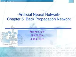
-Artificial Neural Network- Chapter 5 Back Propagation Network. 朝陽科技大學 資訊管理系 李麗華 教授. H 1. Y 1. X 1. Y 2. X 2. H 2. ‧ ‧ ‧. ‧ ‧ ‧. H h. ‧ ‧ ‧. ‧ ‧ ‧. Introduction (1). BPN = Back Propagation Network BPN is a layered feedforward supervised network.

E N D
-Artificial Neural Network-Chapter 5 Back Propagation Network 朝陽科技大學 資訊管理系 李麗華 教授
H1 Y1 X1 Y2 X2 H2 ‧ ‧ ‧ ‧ ‧ ‧ Hh ‧ ‧ ‧ ‧ ‧ ‧ Introduction (1) • BPN = Back Propagation Network • BPN is a layered feedforward supervised network. • BPN provides an effective means of allowing a computer to examine data patterns that may be incomplete or noisy. • Architecture: θ1 θ2 Yj Xn θh
Introduction (2) • Input layer: [X1,X2,….Xn]. • Hidden layer: can have more than one layer. • derive: net1, net2, …neth; transfer output H1, H2,…,Hh, to be used as the input to derive the result for output layer • Output layer: [Y1,…Yj]. • Weights: Wij. • Transfer function: Nonlinear Sigmoid function (*) The nodes in the hidden layers organize themselves in a way that different nodes learn to recognize different features of the total input space.
Processing Steps (1) Briefly describe the processing Steps as follows. • Based on the problem domain, set up the network. • Randomly generate weights Wij. • Feed a training set, [X1,X2,….Xn], into BPN. • Compute the weighted sum and apply the transfer function on each node in each layer. Feeding the transferred data to the next layer until the output layer is reached. • The output pattern is compared to the desired output and an error is computed for each unit.
Processing Steps (2) 5. Feedback the error back to each node in the hidden layer. • Each unit in hidden layer receives only a portion of total errors and these errors then feedback to the input layer. • Go to step 4 until the error is very small. • Repeat from step 3 again for another training set.
x1 θ1 θj H1 net1 Wih : : Yj Whj : : Xi neth Hh : : θh Xn Computation Processes(1/10) • The detailed computation processes of BPN. • Set up the network according to the input nodes and the output nodes required. • Randomly assigned the weights. • Feed the training pattern (set) into the network and do the following computation.
Computation Processes(2/10) 4. Compute from the Input layer to hidden layer for each node. 5. Compute from the hidden layer to output layer for each node.
Computation Processes(3/10) 6. Calculate the total error & find the difference for correction δj=Yj(1-Yj)( Tj -Yj) δh=Hh(1- Hh) ΣjWhj δj 7. ΔWhj=ηδj Hh ΔΘj = -ηδj ΔWih=ηδh Xi ΔΘh= -ηδh 8. update weights Whj=Whj+ΔWhj,Wih=Wih+ΔWih, Θj= Θj + ΔΘj,Θh= Θh + ΔΘh 9. Repeat steps 4~8, until the error is very small. 10.Repeat steps 3~9, until all the training patterns are learned.
W11 H1 X1 W13 W21 Θ1 Y1 W12 Θ3 H2 W23 X2 W22 Θ2 EX: Use BPN to solve XOR (1) • Use BPN to solve the XOR problem • Let W11=1, W21= -1, W12= -1, W22=1, W13=1, W23=1, Θ1=1, Θ2=1,Θ3=1, η=10
EX: BPN Solve XOR (2) • ΔW12=ηδ1 X1 =(10)(-0.018)(-1)=0.18 • ΔW21=ηδ1 X2 =(10)(-0.018)(-1)=0.18 • ΔΘ1 =-ηδ1 = -(10)(-0.018)=0.18 • 以下為第一次修正後的權重值. 1.18 X1 0.754 0.82 0.82 1.915 0.754 X2 1.18
BPN Discussion • Number of hidden nodes increase, the convergence will get slower. But the error can be minimized • The general concept of designing the number of hidden node uses: # of hidden nodes=(Input nodes + Output nodes)/2, or # of hidden nodes=(Input nodes * Output nodes)1/2 • Usually, 1~2 hidden layer is enough for learning a complex problem. Too many layers will cause the learning very slow. When the problem is hyper-dimension and very complex, then we add an extra layer. • Learning rate, η, usually set as [0.5, 1.0], but it depends on how fast and how detail the network shall learn.
The Gradient Steepest Descent Method(SDM) (1) • The gradient steepest descent method • Recall: • We want the difference of computed output and expected output getting close to 0. • Therefore, we want to obtain so that we can update weights to improve the network results.
The Gradient Steepest Descent Method(SDM) (6) • Learning computation