LECTURE 7: Algorithms design techniques - Decrease and conquer -
LECTURE 7: Algorithms design techniques - Decrease and conquer -. Outline. What is an algorithm design technique ? Brute force technique Decrease-and-conquer technique Recursive algorithms and their analysis Applications of decrease-and-conquer. What is an algorithm design technique ?.

LECTURE 7: Algorithms design techniques - Decrease and conquer -
E N D
Presentation Transcript
LECTURE 7: Algorithms design techniques - Decrease and conquer - Algorithmics - Lecture 7
Outline • What is an algorithm design technique ? • Brute force technique • Decrease-and-conquer technique • Recursive algorithms and their analysis • Applications of decrease-and-conquer Algorithmics - Lecture 7
What is an algorithm design technique ? … it is a general approach to solve problems algorithmically … it can be applied to a variety of problems from different areas of computing Algorithmics - Lecture 7
Why do we need to know such techniques ? … they provide us guidance in designing algorithms for new problems … they represent a collection of tools useful for applications Algorithmics - Lecture 7
Which are the most used techniques ? • Brute force • Decrease and conquer • Divide and conquer • Greedy technique • Dynamic programming • Backtracking Algorithmics - Lecture 7
Brute force … it is a straightforward approach to solve a problem, usually directly based on the problem’s statement … it is the easiest (and the most intuitive) way for solving a problem … algorithms designed by brute force are not always efficient Algorithmics - Lecture 7
Brute force Examples: • Compute xn, x is a real number and n a natural number Idea: xn = x*x*…*x (n times) Efficiency class (n) Power(x,n) p:=1 FOR i:=1,n DO p:=p*x ENDFOR RETURN p Algorithmics - Lecture 7
Brute force Examples: • Compute n!, n a natural number (n>=1) Idea: n!=1*2*…*n Efficiency class (n) Factorial(n) f:=1 FOR i:=1,n DO f:=f*i ENDFOR RETURN f Algorithmics - Lecture 7
Decrease and conquer Basic idea: exploit the relationship between the solution of a given instance of a problem and the solution of a smaller instance of the same problem. By reducing successively the problem’s dimension we eventually arrive to a particular case which can be solved directly. Motivation: • such an approach could lead us to an algorithm which is more efficient than a brute force algorithm • sometimes it is easier to describe the solution of a problem by referring to the solution of a smaller problem than to describe explicitly the solution Algorithmics - Lecture 7
Decrease and conquer Example. Let us consider the problem of computing xn for n=2m, m>=1 Since x*x if m=1 x2^m= x2^(m-1)*x2^(m-1) if m>1 It follows that we can compute x2^m by computing: p:=x*x=x2 p:=p*p=x2*x2=x4 p:=p*p=x4*x4=x8 …. Algorithmics - Lecture 7
Decrease and conquer • Analysis: • Correctness • Loop invariant: p=x2^i • b) Efficiency • (i) problem size: m • (ii) dominant operation: * • T(m) = m • Remark: • m=lg n Power2(x,m) p:=x*x FOR i:=1,m-1 DO p:=p*p ENDFOR RETURN p Bottom up approach (start with the smallest instance of the problem) Algorithmics - Lecture 7
Decrease and conquer x*x if n=2 x^n = xn/2*xn/2 if n>2 x*x if m=1 x2^m= x2^(m-1)*x2^(m-1) if m>1 power3(x,m) IF m=1 THEN RETURN x*x ELSE p:=power3(x,m-1) RETURN p*p ENDIF power4(x,n) IF n=2 THEN RETURN x*x ELSE p:=power4(x,n DIV 2) RETURN p*p ENDIF decrease by a constant factor decrease by a constant Algorithmics - Lecture 7
Decrease and conquer power4(x,n) IF n=2 THEN RETURN x*x ELSE p:=power4(x,n DIV 2) RETURN p*p ENDIF power3(x,m) IF m=1 THEN RETURN x*x ELSE p:=power3(x,m-1) RETURN p*p ENDIF • Remarks: • Top-down approach (start with the largest instance of the problem) • Both algorithms are recursive algorithms Algorithmics - Lecture 7
Decrease and conquer The idea of solving the problem can be extended to an arbitrary n as follows x*x if n=2 x^n= xn/2*xn/2 if n>2, n is even x(n-1)/2*x(n-1)/2*x if n>2, n is odd power5(x,n) IF n=1 THEN RETURN x ELSE IF n=2 THEN RETURN x*x ELSE p:=power5(x,n DIV 2) IF n MOD 2=0 THEN RETURN p*p ELSE RETURN p*p*x ENDIF ENDIF ENDIF Algorithmics - Lecture 7
Outline • What is an algorithm design technique ? • Brute force technique • Decrease-and-conquer technique • Recursive algorithms and their analysis • Applications of decrease-and-conquer Algorithmics - Lecture 7
Recursive algorithms • Definitions • Recursive algorithm = an algorithm which contains at least one recursive call • Recursive call = call of the same algorithm either directly (algorithm A calls itself) or indirectly (algorithm A calls algorithm B which calls algorithm A) • Remarks: • The cascade of recursive calls is similar to an iterative processing • Each recursive algorithm must contain a particular case for which it returns the result without calling itself again • The recursive algorithms are easy to implement but their implementation is not always efficient (due to the supplementary space on the program stack needed to deal with the recursive calls) Algorithmics - Lecture 7
Recursive calls - example stack = [] fact(4) 24 fact(4): stack = [4] 4*6 4*fact(3) stack = [4] fact(3): stack = [3,4] fact(3) 6 3*fact(2) 3*2 fact(2): stack = [2,3,4] stack = [3,4] fact(2) 2 2*fact(1) 2*1 fact(1): stack = [1,2,3,4] fact(1) 1 fact(n) If n<=1 then rez:=1 else rez=fact(n-1)*n endif return rez Back to the calling function Recursive call Algorithmics - Lecture 7
Recursive algorithms - correctness • Correctness analysis. • to prove that a recursive algorithm is correct it suffices to show that: • The recurrence relation which describes the relationship between the solution of the problem and the solution for other instances of the problem is correct (from a mathematical point of view) • The algorithm implements in a correct way the recurrence relation • Since the recursive algorithms describe an iterative process the correctness can be proved by identifying an assertion (similar to a loop invariant) which has the following properties: • It is true for the particular case • It remains true after the recursive call • For the actual values of the algorithm parameters It implies the postcondition Algorithmics - Lecture 7
Recursive algorithms-correctness Example. P: a,b naturals, a<>0; Q: returns gcd(a,b) Recurrence relation: a if b=0 gcd(a,b)= gcd(b, a MOD b) if b<>0 Invariant property: rez=gcd(a,b) Particular case: b=0 => rez=a=gcd(a,b) After the recursive call: since for b<>0 gcd(a,b)=gcd(b,a MOD b) it follows that rez=gcd(a,b) Postcondition: rez=gcd(a,b) => Q gcd(a,b) IF b=0 THEN rez:= a ELSE rez:=gcd(b, a MOD b) ENDIF RETURN rez Algorithmics - Lecture 7
Recursive algorithms - efficiency • Steps of efficiency analysis: • Establish the problem size • Choose the dominant operation • Check if the running time depends only on the problem size or also on the properties of input data (if so, the best case and the worst case should be analyzed) • (Particular for recursive algorithms) • Set up a recurrence relation which describes the relation between the running time corresponding to the problem and that corresponding to a smaller instance of the problem. Establish the initial value (based on the particular case) • Solve the recurrence relation Algorithmics - Lecture 7
Recursive algorithms - efficiency Remark: Recurrence relation Algorithm design Recursive algorithm Efficiency analysis Recurrence relation Algorithmics - Lecture 7
Recursive algorithms - efficiency The recurrence relation for the running time is: c0 if n=n0 T(n)= T(h(n))+c if n>n0 rec_alg (n) IF n=n0 THEN <P> ELSE rec_alg(h(n)) ENDIF Assumptions: • <P> is a processing step of constant cost (c0) • h is a decreasing function and it exists k such that h(k)(n)=h(h(…(h(n))…))=n0 • The cost of computing h(n) is c Algorithmics - Lecture 7
Recursive algorithms - efficiency Problem dimension: n Dominant operation: multiplication Recurrence relation for the running time: 0 n=1 T(n)= T(n-1)+1 n>1 Computing n!, n>=1 Recurrence relation: 1 n=1 n!= (n-1)!*n n>1 Algorithm: fact(n) IF n<=1 THEN RETURN 1 ELSE RETURN fact(n-1)*n ENDIF Algorithmics - Lecture 7
Recursive algorithms - efficiency Methods to solve the recurrence relations: • Forward substitution • Start from the particular case and construct terms of the sequence • Identify a pattern in the sequence and infer the formula of the general term • Prove by direct computation or by mathematical induction that the inferred formula satisfies the recurrence relation • Backward substitution • Start from the general case T(n) and replace T(h(n)) with the right-hand side of the corresponding relation, then replace T(h(h(n))) and so on until we arrive to the particular case • Compute the expression of T(n) Algorithmics - Lecture 7
Recursive algorithms - efficiency Example: n! 0 n=1 T(n)= T(n-1)+1 n>1 Forward substitution T(1)=0 T(2)=1 T(3)=2 …. T(n)=n-1 It satisfies the recurrence relation Backward substitution T(n) =T(n-1)+1 T(n-1)=T(n-2)+1 …. T(2) =T(1)+1 T(1) =0 ------------------------- (by adding) T(n)=n-1 Remark: same efficiency as of the brute force algorithm ! Algorithmics - Lecture 7
Recursive algorithms - efficiency power4(x,n) IF n=2 THEN RETURN x*x ELSE p:=power4(x,n/2) RETURN p*p ENDIF Example: xn, n=2m, 1 n=2 T(n)= T(n/2)+1 n>2 T(2m) =T(2m-1)+1 T(2m-1) =T(2m-2)+1 …. T(2) =1 ------------------------- (by adding) T(n)=m=lg n Algorithmics - Lecture 7
Recursive algorithms - efficiency Remark: for this example the decrease and conquer algorithm is more efficient than the brute force algorithm Explanation: xn/2 is computed only once. If it would be computed twice then …it is no more decrease and conquer . pow(x,n) IF n=2 THEN RETURN x*x ELSE RETURN pow(x,n/2)*pow(x,n/2) ENDIF T(2m) =2T(2m-1)+1 T(2m-1) =2T(2m-2)+1 |*2 T(2m-2) =2T(2m-3)+1 |*22 …. T(2) =1 |*2m-1 ------------------------- (by adding) T(n)=1+2+22+…+2m-1=2m-1= n-1 1 n=2 T(n)= 2T(n/2)+1 n>2 Algorithmics - Lecture 7
Outline • What is an algorithm design technique ? • Brute force • Decrease-and-conquer technique • Recursive algorithms and their analysis • Applications of decrease-and-conquer Algorithmics - Lecture 7
Applications of decrease-and-conquer Example 1: generating all n! permutations of {1,2,…,n} Idea: the k! permutations of {1,2,…,k} can be obtained from the (k-1)! permutations of {1,2,…,k-1} by placing the k-th element successively on the first position, second position, third position, … k-th position. Placing k on position i is realized by swapping k with i. Algorithmics - Lecture 7
Generating permutations Illustration for n=3 (top-down approach) 1 2 3 k=3 3↔3 3↔1 3↔2 k=2 1 2 3 3 2 1 1 3 2 3↔3 2↔1 2↔2 2↔2 3↔1 2↔3 1 2 3 k=1 3 2 1 3 1 2 1 3 2 2 1 3 2 3 1 recursive call return Algorithmics - Lecture 7
Generating permutations • Let x[1..n] be a global array (accessed by all functions) containing at the beginning the values (1,2,…,n) • The algorithm has a formal parameter, k. It is called for k=n. • The particular case corresponds to k=1, when a permutation is obtained and it is printed. perm(k) IF k=1 THENWRITE x[1..n] ELSE FOR i:=1,k DO x[i] ↔x[k] perm(k-1) x[i] ↔x[k] ENDFOR ENDIF Remark: the algorithm contains k recursive calls Efficiency analysis: Problem size: k Dominant operation: swap Recurrence relation: 0 k= 1 T(k)= k(T(k-1)+2) k>1 Algorithmics - Lecture 7
Generating permutations 0 k=1 T(k)= k(T(k-1)+2) k>1 T(k) =k(T(k-1)+2) T(k-1)=(k-1)(T(k-2)+2) |*k T(k-2)=(k-2)(T(k-3)+2) |*k*(k-1) … T(2) =2(T(1)+2) |*k*(k-1)*…*3 T(1) =0 |*k*(k-1)*…*3*2 ------------------------------------------------------ T(k)=2(k+k(k-1)+ k(k-1)(k-2)+…+k!) =2k!(1/(k-1)!+1/(k-2)!+…+ ½+1) -> 2e k! (for large values of k). For k=n => T(n) (n!) Algorithmics - Lecture 7
Towers of Hanoi Hypotheses: • Let us consider three rods labeled S (source), D (destination) and I (intermediary). • Initially on the rod S there are n disks of different sizes in decreasing order of their size: the largest on the bottom and the smallest on the top Goal: • Move all disks from S to D using (if necessary) the rod I as an auxiliary Restriction: • We can move only one disk at a time and it is forbidden to place a larger disk on top of a smaller one Algorithmics - Lecture 7
Towers of Hanoi Initial configuration S I D Algorithmics - Lecture 7
Towers of Hanoi Move 1: S->D S I D Algorithmics - Lecture 7
Towers of Hanoi Move 2: S->I S I D Algorithmics - Lecture 7
Towers of Hanoi Move 3: D->I S I D Algorithmics - Lecture 7
Towers of Hanoi Move 4: S->D S I D Algorithmics - Lecture 7
Towers of Hanoi Move 5: I->S S I D Algorithmics - Lecture 7
Towers of Hanoi Move 6: I->D S I D Algorithmics - Lecture 7
Towers of Hanoi Move 7: S->D S I D Algorithmics - Lecture 7
Towers of Hanoi Idea: • move (n-1) disks from the rod S to I (using D as auxiliary) • move the element left on S directly to D • move the (n-1) disks from the rod I to D (using S as auxiliary) • Significance of parameters: • First parameter: number of disks to be moved • Second parameter: source rod • Third parameter: destination rod • Fourth parameter: auxiliary rod • Remark: • The algorithm contains 2 recursive calls Algorithm: hanoi(n,S,D,I) IF n=1 THEN “move from S to D” ELSE hanoi(n-1,S,I,D) “move from S to D” hanoi(n-1,I,D,S) ENDIF Algorithmics - Lecture 7
Towers of Hanoi Illustration for n=3. hanoi(3,s,d,i) s->d hanoi(2,s,i,d) hanoi(2,i,d,s) s->i i->d hanoi(1,s,d,i) hanoi(1,d,i,s) hanoi(1,i,s,d) hanoi(1,s,d,i) s->d d-> i s->d i->s Algorithmics - Lecture 7
Towers of Hanoi T(n) =2T(n-1)+1 T(n-1)=2T(n-2)+1 |*2 T(n-2)=2T(n-3)+1 |*22 … T(2) =2T(1)+1 |*2n-2 T(1) =1 |*2n-1 ---------------------------------------------- T(n)=1+2+…+2n-1 = 2n -1 T(n)(2n) hanoi(n,S,D,I) IF n=1 THEN “move from S to D” ELSE hanoi(n-1,S,I,D) “move from S to D” hanoi(n-1,I,D,S) ENDIF Problem size: n Dominant operation: move Recurrence relation: 1 n=1 T(n)= 2T(n-1)+1 n>1 Algorithmics - Lecture 7
Decrease and conquer variants • Decrease by a constant • Example: n! (n!=1 if n=1 n!=(n-1)!*n if n>1) • Decrease by a constant factor • Example: xn (xn=x*x if n=2 xn=xn/2*xn/2 if n>2, n=2m) • Decrease by a variable • Example: gcd(a,b) (gcd(a,b)=a if a=b gcd(a,b)=gcd(b,a-b) if a>b gcd(a,b)=gcd(a,b-a) if b>a) • Decrease by a variable factor • Example: gcd(a,b) ( gcd(a,b)=a if b=0 gcd(a,b)=gcd(b,a MOD b) if b<>0) Algorithmics - Lecture 7
Next lecture will be on … … divide and conquer … and its analysis Algorithmics - Lecture 7