Download
1 / 58
620 likes | 825 Vues
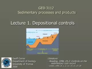
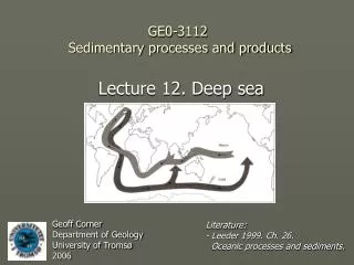
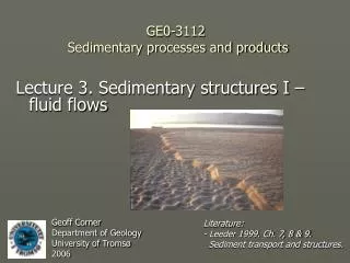
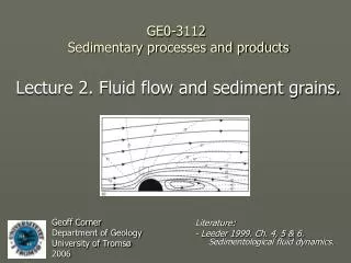
Lecture 2. Fluid flow and sediment grains. GE0-3112 Sedimentary processes and products. Geoff Corner Department of Geology University of Tromsø 2006. Literature: - Leeder 1999. Ch. 4, 5 & 6. Sedimentological fluid dynamics. Contents. 2.1 Introduction - Why study fluid dynamics

E N D
Lecture 2. Fluid flow and sediment grains. GE0-3112 Sedimentary processes and products Geoff Corner Department of Geology University of Tromsø 2006 Literature: - Leeder 1999. Ch. 4, 5 & 6. Sedimentological fluid dynamics.
Contents • 2.1 Introduction - Why study fluid dynamics • 2.2 Material properties • 2.3 Fluid flow • 2.4 Turbulent flow • Further reading
2.1 Introduction - Fluid dynamics • Concerns how fluids transport sedimentary particles. (NB. Fluids are liquids and gasses) • Fluid flows can be described using basic physics, although sedimentary particles add complication.
Why study fluid dynamics? • Examples of practical problems • Pebbles on a sandy surface • Slidden boulder in Death Valley • Deformation structure
Notes on scientific notation • Fundamental units of physical dimension (dimensional analysis): M (mass), L (length), T (time). • System of units of measurement: • Metre-kilogram-second (SI, Systèm Internationale d’Unités). • CGS, centimetre-gram-second (informal) • Greek letters (used in formulas).
2.2 Material properties • Three states of matter (solid, liquid, gas); have different properties and behaviour. • Solids (e.g. rock, ice): have strength and resist shear (limited ...deformation). • Liquids (e.g. water): deform readily under shear stress; incompressible. • Gasses (e.g. air): deform readily under shear stress; compressible • NB. Some substances have behaviour intermediate between liquid and solid (e.g. mud-water mixtures).
Material properties of fluids • Density • Viscosity Density and viscosity are temperature dependent.
Density • Density (ρ) is mass (m) per unit volume [ML-3; kg/m3]. • Solids (rock, ice, sediments) have strength and resist shear (limited ...deformation). • Liquids (water) deform readily under shear stress but are incompressible. • Gasses (air) deform readily under shear stress and are compressible. • NB. Some substances have behaviour intermediate between liquid and solid (e.g. mud-water mixtures). • Density affects:
Density affects: • Fluid momentum • Buoyancy (density ratio)
Density vs. temperature and pressure • Water density decreases with temperature (above 4oC) and increases with pressure. • Air density decreases with temperature and increases with pressure. Water Air
Density vs. salinity • Water density inceases with salinity. • Salinity examples: • Freshwater lakes Norway: <c. 0.4‰ • Brackish water fjords Norway: c. 29-3‰ • Coastal seawater Norway: 33-29‰ • Seawater tropics: 34-35‰
Example 2a: saline stratification in fjords Syvitski 1987
Example 2b: density driven thermohaline circulation in the ocean • Example of flow generated by density and temperature differences: thermohaline flow
Density vs. sediment content • Density increases with sediment content
Example 3: Hypo- and hyperpycnal flows beyond river mouths • Hypopycnal = less dense • Hyperpycnal = more dense • Density differences between the inflowing and ambient water can be caused by a combination of temperature, salinity and sediment concentration differences.
Viscosity • Dynamic (or molecular) viscosity (μ): [ML-1T-1; kg/m s, or N s/m2] (A measure of a fluid’s ability to resist deformation) • Kinematic viscosity (ν): • v=μ/ [L2T-1; m2/s] (Ratio between a fluid’s ability to resist deformation and its resistance to acceleration)
Dynamic (molecular) viscosity • Viscosity controls the rate of deformation by an applied shear, or: • Viscosity is the proportionality factor that links shear stress to rate of strain: • Dimensions are: [ML-1T-1; kg/m s] • Viscosity is much higher in water than in air. Strain rate Shear stress (tau) Viscosity (mu)
Viscosity vs. temperature • Viscosity varies temperature: • In water it decreases. • In air it increases.
Viscosity vs. sediment concentration • Fluid viscosity increases with sediment content.
Viscosity vs. shear rate (Newtonian and Non-Newtonian behaviour) • Newtonian fluids: • Constant viscosity at constant temperature and pressure. • Continuous deformation (irrecoverable strain) as long as shear is maintained. • Non-Newtonian fluids: • Viscosity varies with the shear rate. • Various types of Non-Newtonian behaviour/substances: • Pseudoplastic, Dilatant, Thixotropic, Rheopectic.
Non-Newtonian behaviour • Pseudoplastic: μ decreases as rate of shear increases. • Dilatant: μ increases as rate of shear increases. • Thixotropic: μ decreases with time as shear is applied. • Rheopectic: μ increases with time as shear is applied.
Increasing viscosity Examples from nature Newtonian viscous fluid Non-Newtonian
2.3 Fluid flow • Flow types • Controlling forces • Dimensionless numbers • Flow steadiness and uniformity • Flow visualisation and flow lines • Laminar and turbulent flow (Reynolds number) • Turbulent flow
Flow types • Newtonian: continuous deformation (irrecoverable strain) as long as shear stress is maintained (linear stress-strain relationship). • Plastic: initial resistance to shear (yield stress) followed by deformation. • Bingham plastic: constant viscosity • Non-Bingham plastic: viscosity varies with shear • Non-Newtonian pseudo-plastic • Non-Newtonian thixotropic • Non-Newtonian dilatant
Fluid flow – driving forces • Momentum-driven flows (externally applied forces) (Gravity and pressure differences drive flows) • Buoyancy-driven flows (Density difference drives flows)
Controlling forces • Buoyancy forces (density controlled) • Viscous forces (viscosity controlled) • Inertial forces (momentum controlled) • Gravitational forces
Dimensionless numbers • Dimensionless ratios provide scale- and unit-independent measures of dynamic behaviour. • Two important ratios in fluid dynamics are: • Reynolds number: ratio of inertial to viscous forces • Froude number: ratio of inertial to gravity forces
Flow steadiness • Relates to change in velocity over time • Steady flow - constant velocity • Unsteady flow – variable velocity Steady flow (e.g. steady turbulent river measured over hours) Unsteady flow (e.g. decelerating turbidity current)
Flow uniformity • Relates to change in velocity over distance • Uniform flow - constant velocity (parallel streamlines) • Non-uniform flow – variable velocity (non-parallel sls) Uniform flow (e.g. in channel) Non-uniform (diverging) flow (e.g. at river mouth)
Flow visualisation - flow lines • Streamline - line tangential to the velocity vector of fluid elements at any instant. • Pathline - trajectory swept out over time (e.g. long exposure of a spot tracer). • Streakline - instantaneous locus of all fluid elements that have passed through the same point in the flow field (e.g. short exposure of a continuously introduced tracer. Streamlines Streaklines Pathlines
Flow visualisation – reference frames Streamlines for flow pattern round an object moving to the left through a stationary fluid (Langrangian velocity field) Streamlines for flow past a stationary object (Eulerian velocity field)
Laminar and turbulent flow • Flow type changes with increasing velocity - from laminar to turbulent. • The relationship is described by the Reynolds number. Rapid pressure drop/ change in flow type.
Reynolds number • Reynolds number (Re) is the the ratio of viscous forces (resisting deformation) to inertial forces (ability of fluid mass to accelerate). • The transition from laminar to turbulent flow occurs at about Re = 500 – 2000. Density Velocity Inertial force Depth Viscous force Molecular viscosity
Flow patterns • Laminar flow: parallel flowlines (low Re). • Turbulant flow: irregular flowlines with eddies and vortices (high Re). Laminar flow Transitional to turbulent flow Streaklines Turbulent flow
Velocity distribution in viscous flows Flow retardation in a boundary layer Plug-like non-Newtonian laminar flow (e.g. debris flow). Parabolic Newtonian laminar flow velocity profile.
2.4 Turbulent flow • Turbulent eddies • Bed roughness • Flow separation
Turbulent eddies Backwash/rip-current eddies at Breivikeidet Eddy movement in x-y space with time (t1-t2)
+η(Boussinesq’s eddy viscosity) Bed roughness Turbulent stresses dominate Viscous sublayer Viscous forces dominate
Bed roughness No viscous sublayer (rough bed) Viscous sublayer (smooth bed)
Shear velocity and skin friction Rough Smooth
Streaklines viewed in the x-z plane (i.e. plan section) Streaklines viewed in the x-y plane (i.e. flow-parallel vertical section) Turbulent eddies in air
Components of turbulent eddies Streaks (close to bed) Sweep (fast) Burst (slow)
Slow flow pattern in viscous sublayer Flow pattern in turbulent boundary layer Flow at successively higher positions above the bed (a- d) Macroturbulence in outer regions of flow Sand particle flow in viscous sublayer shown at 1/12 s time intervals ’Sweep’ event Turbulent eddies in water
Kelvin-Helmholz vortices • Important mixing mechanism at junction of two fluids, e.g. at junctions of tributaries or mixing water masses, at fronts and tops of density currents, etc. Likely causes of K-H instability: a)-c) velocty differences across boundary layer or in density-stratified flows; d)-e) shear layers produced by pressure differences.
Flow separation Boundary layer separation point Boundary layer reattachment zone (downstream)
Decelerating flow, increasing pressure, redardation and separation of flow closest to the bed Accelerating flow, decreasing pressure
2.5 Sediment grains in fluids • Settling (Stokes velocity) • Threshold velocity • Rolling, saltation and suspension • Bedload, suspended and washload