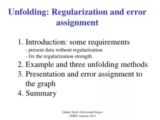
Unfolding: Regularization and error assignment

1. Unfolding: Regularization and error assignment • Introduction: some requirements • - present data without regularization • - fix the regularization strength • 2. Example and three unfolding methods • 3. Presentation and error assignment to the graph • 4. Summary Günter Zech, Universität Siegen CERN, January 2011

2. The problem standard unfolding unknown true distribution true data sample observed data sample Poisson binning-free unfolding smearing We got y, we want to know f(x) We parametrize the true distribution as a histogram (there are other attractive possibilities, i.e. splines) Günter Zech, Universität Siegen CERN, January 2011

3. As has been stressed, unfolding belongs to the class of illposed problems. Howeves when you parametrize the true distribution as a histogram with given bin widths, the problem becomes defined. We then can determine the parameters of the bins and the corresponding error matrix. This is our mesurement which summarizes the information contained in the data. The errors have to allow for all distributions that are compatible with the observed data. Günter Zech, Universität Siegen CERN, January 2011

4. Even in the limit of infinite statistics unfolding does not necessarily lead to the correct solution. Example: N(0,1) folded with N(0,1), avoiding statistical fluctuations. smeared distribution original distribution result of unfolding (MLE) Increasing the statistics would add further delta function peaks Günter Zech, Universität Siegen CERN, January 2011

5. Unfolding without regularization, the errors are strongly correlated. The error matrix has to be provided. This is from an example to be discussed in more detail below Günter Zech, Universität Siegen CERN, January 2011

6. Many unfolding issues outside physics are directed towards the point estimate (unblurring pictures) and the interval estimation is of minor importance. In particle physics it is the other way round. • Essential requirements • All measurements have to be presented in such a way that they can be combined with other measurements. They have to be associated with error limits that permit to check the validity of theoretical predictions. This applies also to data that are distorted by measurement errors.  Publish data without regularization. • In addition we also need a graphical presentation.  Regularization Günter Zech, Universität Siegen CERN, January 2011

7. Three alternative proposals for requirement 1: • Unfold result without regularization and publishwith full error matrix. • Determine eigenfunctions of the LS matrix. Publish these functions together with the uncorrelated fitted weights and corresponding errors. • Publish observed data with their uncertainties together with the smearing matrix. • The first approach works only with reasonably large statistics (normally distributed errors of the unfolded bin entries.) • The third method leaves all the work to the user of the data. Günter Zech, Universität Siegen CERN, January 2011

8. Problem 2, regularization: There is no general rule, how to smooth the data, but the result has to be compatible with the data. (Clearly, some methods make more sense than others.) The choice of the regularization method is subjective (in priciple Bayesian). Smoothing is always related to a loss of information. Thus unfolded distributions with regularization are not well suited to discriminate between theories (Cousins‘ requirement cannot be fulfilled except in special situations.) Regularization introduces constraints and for that reason reduces the nominal values of the errors. There is nothing strange about obtaining error < SQRT (number of events). Günter Zech, Universität Siegen CERN, January 2011

9. How to fix the regularization strength? Proposal: The regularization strength should be fixed by a commonly accepted p-value based on a goodness-of-fit statistic (normally c2) The smoothed result has to be compatible with the observed data and this means to the fit without regularization. The fit without regularization is the measurement. Günter Zech, Universität Siegen CERN, January 2011

10. schematic illustration with 2 true bins, p-value 90 %. Günter Zech, Universität Siegen CERN, January 2011

11. = c2without regularization p = p-value, uN = c2 distribution for N degrees of freedom, N = number of true bins For an error ellipse corresponding to a 1-p confidence interval centered at the parameters computed without regularization the parameters with regularization is located at the surface. Important: do not use the nacked c2reg value of the observed distribution to compute the p value! It is not relevant. We are not checking the goodness-of-fit but want the regualized solution to be compatible with the standard fit. Proposal: require p > 90 % (The reg. solution is close to the solution without regularization.) Günter Zech, Universität Siegen CERN, January 2011

12. Some common unfolding and regularization methods Notation: true distribution: underlying theoretical distribution, described by vector q original or undistorted histogram: ideal histogram before smearing, and acceptance losses, described by vector c observed or data histogram: includes experimental effects, described by vector (estimate of the expected value d) Smearing matrixT: includes acceptance losses d = T q Günter Zech, Universität Siegen CERN, January 2011

13. q true distribution / histogram Poisson process c original histogram E(c ) = q smearing and acceptance process T observed histogram, d = Tq Günter Zech, Universität Siegen CERN, January 2011

14. We use the following example: superposition of : 2500 events N(0.3;0.1) 1500 events N(0.75;0.08) 1000 uniform events = 5000 events Gaussian resolution N(0;0.07) observed distribution: 40 bins true distribution: 20 or 10 bins 0 1 In this example a rather bad resolution was chosen to amplify the problems. Günter Zech, Universität Siegen CERN, January 2011

15. 1. c2 fit of the true distribution, eliminate insignificant contributions (SVD) (LSF), minimize c2, Gaussian approximation linearized approximation (used in matrix LSF, SVD ) Günter Zech, Universität Siegen CERN, January 2011

16. In matrix notation (see for example Blobel‘s note): The least square fit has to include the error matrix E of the data vector d. (weight matrix V=E-1). T is rectangular, we transform it to a quadratic matrix C: The eigenvectors ui of C are uncorrelated, q = Sciui Günter Zech, Universität Siegen CERN, January 2011

17. u1 eigenvectors ui The true distribution is a superposition of these functions, ordered with decreasing eigenvalues. The coefficients (parameters) ci are fitted. Cut on significance = |parameter/error| = |ci/Dci| u20 Günter Zech, Universität Siegen CERN, January 2011

18. Unfolding result for different cuts in significance Where should we cut? Günter Zech, Universität Siegen CERN, January 2011

19. Remarks: • small eigenvalues are not always correlated with insignificant parameters • cutting at 1 st. dev. produces unacceptable results, better cut at p=0.9 • the errors decrease with increased regularization strength. In graphs F and G some errors are smaller than SQRT(number of events), symmetric errors are not adequate. E F G Günter Zech, Universität Siegen CERN, January 2011

20. same thing for 10 bins Günter Zech, Universität Siegen CERN, January 2011

21. With 10 bins, regularization is not necessary. Günter Zech, Universität Siegen CERN, January 2011

22. 2.Poisson likelihood fit with penalty regularization for a single bin i with expectation di: for the histogram with penalty term R: Frequently used penalty term Günter Zech, Universität Siegen CERN, January 2011

23. Standard: curvature regularization prefers a linear distribution. r: regularisation strength You can use a different penalty term and apply for instance the regularization to the deviation of the fitted from the expected shape of the distribution (iterate). For a nearly exponential distribution: We could also normalize the expressions to the expected uncertainty. Günter Zech, Universität Siegen CERN, January 2011

24. Günter Zech, Universität Siegen CERN, January 2011

25. For 10 true bins p=0.997 p=0.54 p=0.87 Günter Zech, Universität Siegen CERN, January 2011

26. c) Iterative LSF (Introduced to HEP by Mültai and Schorr 1986, see refs.) Inverts the relation d = Tq iteratively (iterative matrix inversion) This is equivalent to the LSF with diagonal and equal errors for the data vector. (However, in principle, the the error matrix could be implemented without major difficulty) Günter Zech, Universität Siegen CERN, January 2011

27. How does it work? Multiply each contribution by a factor to get agreement with the observed distribution and put it back into the true distribution. Günter Zech, Universität Siegen CERN, January 2011

28. Folding step: Unfolding step: ei: efficiency of bin i Günter Zech, Universität Siegen CERN, January 2011

29. Günter Zech, Universität Siegen CERN, January 2011

30. Günter Zech, Universität Siegen CERN, January 2011

31. Comparison of Poisson likelihood with curvature regularization to iterative unfolding. The results in the limit of no regularization are nearly identical. Günter Zech, Universität Siegen CERN, January 2011

32. D‘Agostini‘s Bayesian unfolding (arXiv:1010.0632v1) Günter Zech, Universität Siegen CERN, January 2011

33. D‘Agostini reconstructs the original histogramc and not the true distribution. This complicates the problem (multinomial distribution). Being unable to write down a Bayesian formula relating the full histogram c and the observation d he applies a “trick“: • use Bayes‘ theoremto relate observed d-bins (effect bins) to individual c-bins (cause bins) with a uniform prior for the c-histogram. • use a polynom fit (or equivalent) to smooth the c-distribution (details do not matter) • use updated c-distribution as prior for next iteration. • By chance this leads to the same iterative process as that introduced by Mültai et al. described above (except for the intermediate smoothing) • Due to the smoothing step, the procedure converges to a smooth distribution. Regularization is inherent in the method. Günter Zech, Universität Siegen CERN, January 2011

34. The error calculation then includes a Poisson error for the d-bins in combination with the multinomial error related to the smearing matrix. • Further ingredients: (The new vesion is consistently Bayesian) • Prior densities are used for the parameters of the multinomial and the Poisson distributions. • The uncertainties of the smearing matrix are taken into account by sampling. Günter Zech, Universität Siegen CERN, January 2011

35. My personal opinion: • There is no need to use the multinomial distribution. Starting from the true distribution, it is possible to introduce a prior in the standard way, but this doesn‘t produce a smooth result. The smoothing is due to the “trick“. • The intermediate smoothing and the related convergeance are somewhat arbitrary (no p-value criterion). • Introducing prior densities for the secondary parameters is unlikeliy to improve the result. • I am not convinced that the error calculation is correct. (Giulio is checking this). • I cannot see an essential advantage in D‘Agostini‘s program compared to the simple iterative method as introduced by Mültai et al. with the aditional c2 stopping criterion. Günter Zech, Universität Siegen CERN, January 2011

36. Comparison of the three unfolding approaches: All three methods produce sensible results • Suppression of “insignificant“ contributions in the LS approach: • mathematically attractive, provides the possibility to document the result without regularization • requires high statistics (normal error distribution), problematic in cases where the true distribution has bins with low number of events  negative entries. • the cut of insignificant contributions is not straight forward. Günter Zech, Universität Siegen CERN, January 2011

37. Poisson likelihood fit with penalty term • works also with low statistics • very transparent • easy to fix the regularization strength • a curvature penalty works well, but not obvious why to choose. The penalty term can be adjusted to specific problem • smoothing even when the data are not smeared! (but this is ok) Günter Zech, Universität Siegen CERN, January 2011

38. Iterative unfolding a la Mültai • technically very simple. • does not require large statistics • offers a sensible way to implement the smoothing prejudices (but a uniform starting distribution always seems to work) • it is not clear why it works so well! Günter Zech, Universität Siegen CERN, January 2011

39. Some further topics • Binning: • The choice of the bin with b of the true distribution depends on • the number of events N • The structure of the distribution s (1/s is typical spatial frequency) • The resolutions • We want narrow bins to reconstruct narrow structures of the true distribution • We want wide bins to have little correlation between neighboring bins. • (Wide bins suppress high frequency oscillations) • Try to fulfil: s < b < s (but sometimes s > s) • For large N we can somewhat relax this requirement, but even with infinite statistics unfolding remains a problematic procedure. Günter Zech, Universität Siegen CERN, January 2011

40. Effect of the shape of the Monte Carlo distribution, flat (black) vs. exact (red) Günter Zech, Universität Siegen CERN, January 2011

41. Statistical uncertainty in the smearing matrix and background contributions. These are purely technical problems. For the statistical uncertainty in the smearing matrix see Blobel‘s report. A simple but computationally more involved method to determine the effects of background and smearing errors is bootstrapping: Take the Monte Carlo event sample (N events) used to determine the smearing matrix. Contruct a bootstrap samply by drawing N events from the sample with replacement. (Some events occur more than once.) . The spread of M unfolding results from M bootstrap smearing matrices indicates the uncertainty. (This is also used by D‘Agostini) Günter Zech, Universität Siegen CERN, January 2011

42. Background can normally be treated in a simpler way: Either add one bin in the true distribution (background bin) and a further column in the smearing matrix which gives the probability to find background in a certain observed bin. (iterative method) or subtract the backgroung in the observed distribution and correct the error matrix of the observed histogram. or subtract the background and estimate the introduced uncertainty by bootstrap from a background sample. Whatever you understand, you can simulate, and what you can simulate, you can correct for, using bootstrap if you don‘t find a simpler way. Günter Zech, Universität Siegen CERN, January 2011

43. Graphical representation of the result • To indicate the shape of the true distribution, we need unfolding with regularization. Standard unfolding methods provide reasonable estimates, however there is a problem with the error estimates. The errors derived from the constained fit or computed by error propagation are arbitrary and misleading and therefore useless. • There is no perfect way to indicate the precision of the unfolded result but a better way to illustrate the quality of the point estimate is the following: • Use as a vertical error bar the statistical error from the effective number of entries in the bin, ignoring correlations. • Indicate by a horzontal bar the resolution of the experiment at the location of the bin. • This procedure permits to estimate qualitatively whether a certain prediction is compatible with the data and is independent from personal prejudices (regularization method and strength.) Günter Zech, Universität Siegen CERN, January 2011

44. Vertical error: SQRT ( effective number of events ) This is similar to the nominal errors uf regularized unfolding in the case where the bins are not correlated. Horizontal bar: resolution. Günter Zech, Universität Siegen CERN, January 2011

45. Summary The measurement should be published in the standard way: point estimate + error matrix (or equivalent, no regularization)  possibility to combine data and compare with theory. For a graphical representation we have to apply regularization. (This introduces constraints, subjective input and implies a loss of information.) The regularization strength should be fixed by a common p-value criterion. This alows to compare different approaches. The errors produced by a fit with regularization exclude distributions with narrow structures which however are compatible with the data. Proposal: Choose errors which are independent from the applied regularization. (effective number of entries + resolution) My preferred unfolding methods are: Poisson likelihood fit + penalty and iterative unfolding with c2 stopping criterion. Günter Zech, Universität Siegen CERN, January 2011

46. References, mainly on iterative unfolding V. Blobel, preliminary report (2020). Y. Vardi and D. Lee, From image deblurring to optimal investments: Maximum likelihood solution for positive linear inverse problems (with discussion), J. R. Ststist. Soc. B55, 569 (1993). L. A. Shepp and Y.Vardi, Maximum likelihood reconstruction for emission tomography, IEEE trans. Med. Imaging MI-1 (1982) 113. Y. Vardi, L. A. Shepp and L. Kaufmann,A statistical model for positron emission tomography, J. Am. Stat.Assoc. (1985) 8. A. Kondor, Method of converging weights - an iterativeprocedure for solving Fredholm's integral equations of the first kind, Nucl. Instr. and Meth. 216 (1983) 177. H. N. Mülthei and B. Schorr, On an iterative method for the unfolding of spectra, Nucl. Instr. and Meth. A257 (1987) 371. G. D'Agostini, A multidimensional unfolding method based on Bayes' theorem, Nucl. Instr. and Meth. A 362 (1995) 487. G. Bohm, G. Zech, Introduction to Statistics and Data Analysis for Physicists, Verlag Deutsches Elektronen-Synchrotron (2010), http://www-library.desy.de/elbook.html(contains also unbinned unfolding). Günter Zech, Universität Siegen CERN, January 2011