Download
1 / 42
420 likes | 469 Vues
Development of new numerical tools, from single to multi-physics, integrating disciplines for concurrent engineering and optimisation. Learn the iterative optimisation process and constraints involved in aerodynamic shape optimisation. Utilize mathematical tools for optimal design.

E N D
Aerodynamic Optimisation V. Selmin Multidisciplinary Computation and Numerical Simulation
Development of a new generation of numerical tools New Trends in Design Drivers: Reduce product development costs and time to market • Single discipline optimisation process • From analysis/verification to design/optimisation • From single to multi-physics • Integration of different disciplines, Interfaces between disciplines, • Concurrent Engineering • Multidisciplinary optimisation process • Integration of different disciplines within the design process, • Optimisation, Concurrent Engineering
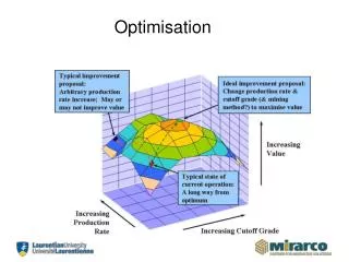
Optimisation Problem To solve the optimisation problem, the values assigned to the design variables must be found so as to minimise the objective function while maintaining that the possible constraint functions are smaller or equal to zero The designer must derive these functions and choose the design variables that govern the transformation of the system to be improved. In the case of aerodynamic shape optimisation, the design variables are related to the transformation the geometry, e.g. wing.
Objective functions and constraints The general aerodynamic design requirements need to be translated into mathematical formulas for constraints and objective functions. A simple expression for the objective function includes the linear combination of aerodynamic coefficients at one or more operating conditions n . For instance, Constraints on the geometry and on its aerodynamic performances may be used. The aerodynamic constraints are used to control the values of the design coefficients (Cl or Cm), while geometric constraints are used to satisfy structural requirements and to indirectly control aerodynamic characteristics in off-design conditions. The following expression may be used for the constraints: The parameter K represents a multiplication factor which is used to give a relative weight to each equation of the constraint set; in general, it is set to be equal to unity.
Problem Definition Problem Definition Initial Models Database Initial Models Database Multi- Models Generation Multi- Models Generation Multidisciplinary Computations Optimisation Algorithm Multidisciplinary Computations Optimisation Algorithm Objective Constraints Objective Constraints Optimised Models Database Optimised Models Database Shape Optimisation System Mathematical tools, such as sensitivity analysis, modelling methods, and optimisation solvers, provide a mechanism by which working together can be accomplished.
Grid Update: • Mesh deformation techniques Parameterisation: • Aerodynamic Analysis: • FV Euler & Navier-Stokes solvers • Unstructured/hybrid grids • Optimisation Algorithm: • Deterministic Methods • Gradient Based methods • (Methods of Feasible Directions, • Sequential Quadratic Programming) • Stochastic Methods • Evolutionary algorithms • Gradient Computation: • Finite differences • Adjoint methods • Automatic differentiation Shape Optimisation System
g2(X)=0 g1(X)=0 Optimisation algorithms: Basic Concepts Unconstrained function minimisation Find the minimum value of the following algebraic function: No limits are imposed on the value of X and no additional conditions must be met for the design to be acceptable. Unconstrained Problem In order to solve the problem, a necessary condition(but not sufficient) is the vanishing of the gradient of the function. Solving for and , it is found Constrained function minimisation The additional functions (constraints) will limit the space of feasible solutions. Constrained Problem
Optimisation algorithms: Basic Concepts General problem statement The non linear constrained optimisation may be written in general as follows: Minimise: objective function Subject to: inequality constraints equality constraints side constraints The functions may be explicit or implicit with respect to the design variables and may be evaluated by any analytical or numerical techniques. It may be important (except for special class of optimisation problems) that the function be continuous and have continuous first derivatives with respect to de design variables. If the equality constraints are explicit in the design variables, they can often be used to reduce the number of design variables considered. Although the side constraints could be included in the inequality constraints, it is usually convenient to treat them separately because they define the region of search for the optimum.
Optimisation algorithms: Basic Concepts Iterative optimisation procedure Most optimisation algorithms require that an initial set of design variables, , be specified. Beginning from this starting point, the design is updated iteratively. The most common form of this iterative procedure is given by The scalar quantity defines the distance that we wish to move in direction S . By searching in a specified direction, the problem has been converted from one in n variables X to one variables . It is seen that this kind of optimisation algorithm can be separated into two basic parts: 1- Determination of a direction of search S , which will improve the objective function subject to constraints. 2- Determination of the scalar parameter defining the distance of travel in direction S. Each of these components plays a fundamental role In the efficiency and reliability of a given optimisation algorithm.
Optimisation algorithms: Basic Concepts Existence and uniqueness of an optimum function In the application of optimisation techniques to design problems of practical interest, it is seldom possible to ensure that the absolute optimum design will be found subject to constraints. This may be because multiple solutions to the optimisation problem exist (relative extrema) or because numerical ill-conditioning in setting up the problem results in extremely slow convergence of the optimisation algorithm. From a practical standpoint, the best approach is usually to start the optimisation process from several different initial vectors, and if the optimisation result is essentially the same final design, one can be reasonably assured that this the true optimum. It is possible to define (mathematically) necessary conditions for an optimum and it can be shown that under certain circumstances these necessary condition is also sufficient to ensure that the solution is the global optimum.
Optimisation algorithms: Basic Concepts Existence and uniqueness of an optimum function: Unconstrained problems A necessary condition for F(X) to be an extremum (minimum/maximum), is that its gradient must vanish F(X) will be a minimum when its Hessian matrix is positive definite. If the gradient is zero and the Hessian matrix is definite positive at a given X , this ensures that the design is at least a relative minimum. The design is only guaranteed to be a global minimum if the Hessian matrix is positive definite for all possible values of the design value X .
Optimisation algorithms: Basic Concepts Existence and uniqueness of an optimum function: Constrained problems It is no longer necessary that the gradient of the objective vanish at the optimum. Starting of a given point, in order to improve on this design, it is necessary to determine a direction vector S that will reduce the objective function and not violate the active constraint. Usable direction: Feasible direction: At the optimum, the gradients of the objective and the constraint point exactly in the opposite directions. The only possible vector S that will satisfy the requirements of usability and feasibility will be precisely tangent both to the constraint boundary and to a surface of constant objective function and will form an angle of 90° with both gradient. This condition can be stated mathematically as
Optimisation algorithms: Basic Concepts Advantages of using numerical optimisation 1- Reduction in design time. 2- Can operate with a wide variety of design variables and constraints which are difficult to visualise. 3- Optimisation virtually always yields some design improvement. 4- It is not biased by intuition or experience in engineering. Therefore, the possibility of obtaining improved, non traditional designs is enhanced. 5- Optimisation requires a minimal amount of human-machine interaction. Limitation of numerical optimisation 1- Computational time increases as the number of design variables increases (depends of the optimisation strategy). 2- Optimisation techniques have no stored experience or intuition on which to draw. They are limited to the range of applicability of the analysis program. 3- If the analysis program is not theoretically precise, the results of optimisation may be misleading, and therefore the results should always be checked very carefully. 4- Most optimisation algorithms have difficulty in dealing with discontinuous functions (not for stochastic methods) 5- It can be guaranteed that the optimisation algorithm will obtain the global design optimum. Stochastic methods may help. Particular care have to be taken in formulating the automated design problem.
Unconstrained minimisation Usable-feasible regions/directions, constrained minimisation Optimisation algorithms: Constraints treatment Direct method Objective function: Inequality constraints: Equality constraints: Augmented objective method Objective function: Modified objective function → modified relative extrema
Optimisation algorithms: Deterministic Methods In general based on the Iterative Optimisation Procedure. 1- Determination of a direction of search S 2- Determination of the scalar parameter by a 1D minimisation procedure along the direction S. Unconstrained Problems: 1- Zero-order methods: Powell method 2- First-order methods: Steepest descent Conjugate direction method 3- Second-order methods: Newton method
Optimisation algorithms: Deterministic Methods Constrained Problems: 1- Linear Programming: Simplex method 2- Sequential Unconstrained Minimisation Techniques: Exterior penalty function method Interior penalty function method 3- Direct methods: Based on the concept of usable/feasible directions Methods of feasible directions Constrained steepest descend method Sequential Linear or Quadratic Programming
Optimisation algorithms: Stochastic Methods Evolutionary Computing Genetic Algorithms/Evolutionary Strategies Evolutionary computing simulates the mechanism of selection and mutation which are typical of the natural evolution in the Darwinian theory. The algorithm uses a string codification of the problem design variables called chromosome. An initial population of possible solutions evolves under the action of selection, crossover and mutation mechanisms applied to chromosomes. The selection is driven by a cost function (fitness) to promote the best fit individuals during the reproduction phase. The crossover scheme arranges genetic information recombination and the mutation mechanism introduces a small random variation in the genetic code. Allow to reach global optima, but very expensive (large number of functional evaluations) Constrained problems issues. Hybrid approach Combining evolutionary computing and gradient based optimisation seems to offer promising perspectives. 1- Move close to the global optima by using evolutionary strategies 2- Continue the search by using a gradient based method (more efficient close to the optima)
Optimisation algorithms: Other issues Surface response During the optimisation process, values of the objective and constraints functions are computed. Use of these values to form approximated functions, by using polynomials approximations or others. These approximated functions may be used instead of direct evaluations during the optimisation process. Multiple objectives, Pareto front Let define the following design problem: Minimise The Pareto front is the envelop of the values of X that satisfy The Pareto front is naturally obtained by using Evolutionary Computing Robust design Solve the optimisation problem in a weak form within an interval of variation of the parameters that define the optimisation problem and by using mean values and variance probabilistic concepts
Spring Analogy: Source terms allow to control mesh quality Algorithm: Differentiation: Grid Update: Mesh deformation
Shape modification Aeroelastic deformation Grid Update: Mesh deformation
Shape Parameterisation The shape of the object to be optimised will be parameterised with respect to the design variables. The choice of the design variables is essential. 1- They will allow to obtain a poor or good design depending of the shape they can allowed. 2- If possible they have to represent quantities that are close to the engineer knowledge/education. 3- For aerodynamics applications, some aerodynamics behaviours are related to particular geometrical features. It could be interesting to have these quantities as design variables. (Linear inequalities as constraints) These could also be related to some semi-empirical knowledge about aerodynamic behaviours. The parameterisation could address: 1- the direct representation of the object. 2- the modification of an initial shape. (Preferred) The transfer of information from the modified shape to the CFD grid has to be addressed in terms of accuracy and flexibility When the design problem is applied to complex shapes, the shape parameterisation problem becomes difficult. A way is to introduce the parameterisation directly into the CAD system. But, that means that the interaction between the overall optimisation system and the CAD has to be easy, which is seldom the case.
Differentiation: Shape Parameterisation Planform Defining Parameters: Area (Sr), Aspect Ratio (AR), Sweep Angle (Sw), Taper Ratios (TR) Wing Section Parameters: Twist (Tw), maximum Thickness(Th) Wing Section Shape Parametrisation: Thickness Distribution + Camberline Modification
Aerodynamic Solver RANS Solver • Node-centred based Finite Volume spatial discretisation • Blended second- and fourth order dissipation operators • Operates on structured, unstructured and hybrid grids • Time integration based on Multistage Algorithm (5 stages) • Residual averaging and local timestepping • Preconditioning for low Mach number • Pointwise Baldwin-Barth, K-Rt (EARSM) turbulence models • Chimera strategy implementation • ALE implementation for moving grid • Time accurate simulation provided by using Dual Timestepping • Scalar, vector and parallel implementation
Finite Volume Discretisation: Differentiation: Aerodynamic Solver Conservation principle: Euler equations Navier-Stokes equations
Cost function U is the state vector X computational grid B design variables vector Differentiation Finite Difference method Cost of gradient evaluation directly proportional to the number of design variables Direct Differentiation Method Gradient Computation
Adjoint Method Adjoint equation: Cost of gradient evaluation independent of the number of design variables But an adjoint equation solution for each state functions. Automatic Differentiation Forward Mode DDM Reverse Mode AM Fortran code of Fortran code of Adifor, Tapenade, ... Gradient Computation
Simulation chain Differentiation Aerodynamic simulation chain and its sensitivity
Automatic Differentiation Forward Mode Reverse Mode Param_d Param_b MeshUpd_d MeshUpd_b Metrics_d Metrics_b Solver_d Solver_b
Software re-engineering: • Organise the software in order to separate pieces of code that have to be differentiated to the other routines. • Sometimes, that means splitting of a code in several codes. • It leads in general to a beneficial effect on the structure of the code and on code efficiency for an iterative process • (optimisation, aeroelasticity,...). • Some optimisation (also manual) can also be necessary in order to avoid redundancies. Efficiency improvement: • Start from a frozen converged state solution • That means to cancel from the differentiated code all the instructions that are not strictly related to • gradient computation • In addition, no more need to compute the timestep derivative Automatic Differentiation
Differentiation with respect to computation parameters RAE2822 airfoil: M=0.75, a=2º
Differentiation with respect to shape parameters NACA0012 airfoil: M=0.50, a=1º M=0.85, a=1º Shape parameters: Xtmax: location of max. thickness Tmax: Value of max. thickness
Multi Point Airfoil Optimisation The problem consists in the improvement of an already existing airfoil in order to increase its maximum speed without deteriorating its characteristics at lower speeds. More precisely, the design problem was defined as to minimise drag at maintaining the characteristics on the buffet onset curve of the original airfoil for which results in a five points optimisation problem. The value of the Reynolds number is
Objective: Design points: Constraints: Transonic Multi Point Airfoil Optimisation
Airfoil geometry Thickness Distribution Camberline M=0.680, a=1.8 M=0.734, a=2.8 M=0.754, a=2.8 Transonic Multi Point Airfoil Optimisation
Supersonic Commercial Aircraft Optimisation Supersonic Aircraft Geometry
Supersonic Commercial Aircraft Optimisation Baseline exercise Optimisation of the fuselage geometry with fixed datum wing geometry Flight conditions : M=2.0, Cl=0.12, AoA free Cost function: minimum drag Design variables: fuselage contraction Demonstration exercise Optimisation of both the fuselage and wing geometry Mandatory test case Flight conditions : M=2.0, Cl=0.12, AoA free Cost function: minimum drag Design variables: fuselage contraction, wing camber, thickness distribution & twist Voluntary test case Flight conditions : M=2.0 , Cl=0.12, AoA free, W=2.0 (supersonic cruise) M=0.95, Cl=0.20, AoA free, W=1.0 (transonic cruise) Cost function: minimum drag, multi-point design Design variables: fuselage contraction, wing camber, thickness distribution & twist Constraints Constraints on spanwise variation of minimum thickness, fuselage incidence, fuselage diameter, minimum lift and pitching moment
Original Optimised M=2.0, Cl=0.12, ΔCd = 2% Supersonic Commercial Aircraft Optimisation Supersonic Commercial Aircraft: Fuselage optimisation
Design variables: Camberline modification (2), Maximum thickness, at 6 master sections Twist, AoA Linear interpolation between the master sections Objective function & Constraints histories: } Supersonic Commercial Aircraft Optimisation Supersonic Commercial Aircraft: Wing optimisation
Supersonic Commercial Aircraft Optimisation Supersonic Commercial Aircraft: Wing optimisation
Supersonic Commercial Aircraft Optimisation Supersonic Commercial Aircraft: Wing optimisation
Supersonic Commercial Aircraft Optimisation Supersonic Commercial Aircraft: Wing optimisation
Summary Optimisation Problem Definition The optimisation problem – objective and constraint functions – have to be accurately defined Optimisation Algorithms Deterministic Methods Stochastic Methods Unconstrained-Constrained problems issues Parametrisation Issues Impact on the optimisation problem solution Impact on the users (basic knowledge, experience) Treatment of complex shapes issues CFD Grid Deformation Issues Maintain the same grid quality during the overall optimisation process. Automated Optimisation System Issues Integration of the system issues Flexibility Robustness of the system Control during the optimisation process