Download

1 / 17
170 likes | 318 Vues
Application of reliability prediction model adapted for the analysis of the ERP system. F rane Urem, K rešimir Fertalj , Željko Mikulić College of Šibenik , Department of management Faculty of Electrical Engineering and Computing, University of Zagreb. Introduction.

E N D
Application of reliability prediction model adapted for the analysis of the ERP system Frane Urem, Krešimir Fertalj, Željko Mikulić College of Šibenik, Department of management Faculty of Electrical Engineering and Computing, University of Zagreb
Introduction • the possibilities of using Weibull statistical distribution in modeling the distribution of defects in ERP systems • a case study, which examines helpdesk records of defects that were reported as the result of one ERP subsystem upgrade • modeling the reliability of the ERP system with estimated parameters like expected maximum number of defects in one day or predicted minimum of defects between two upgrades
Measurement-based analysis framework of ERP system reliability
Step 1 • defects grouped in samples by days for every period between upgrades (month) • e.g. the 7th month, Module1 • samplesize N = 22 • number of bins (k)≈ 6 • max defects/day, Dmax = 26 • width of interval that includes num. of defects in separate bins (1) = 5 (2)
Step 2 • as a result of (1) and (2), defects from T1 are sorted at T2 as empirical distribution of number of defects from T1
Step 3 • analysis of data has resulted in Weibull distribution of number of defects for every period between two subsequent upgrades • e.g. theoretical best fit Weibull distribution • for empirical distribution from Table 2 • calculated with EasyFit [3] • with parameters α=1,9797, β=13,752
Step 4 • Theoretical Weibull distribution • n is number of defects • P(n) is cumulative probability for number of defects that will be distributed in interval [0,n] • Comparison • empirical and best fit Weibull distribution, Module1, 7th month • n=25, α=1,9797, β=13,752
Step 5 • prediction of future values of the theoretical distributions based on previous reports • Linear Regression (LR), α=1,9933; β=11,6138 • k Nearest Neighbors (kNN), α=1,8762; β=12,9642 • Kolmogorov-Smirnov (KS) and Anderson-Darling (AD) test • significance level (α=0,05), typical for tech. applications
Case study (1) • telecom operator, help desk, monthly upgrades • proving that all empirical distributions of the number of defects identified after the completion of upgrades can be described with theoretical Weibull distributions
Case study (2) • explore the possibility of predicting distributions • predictions made for periods after 4th month (following table) • KNN algorithm was used with parameter k = 3, there was no point in predicting earlier because that version of KNN algorithm needs a minimum of three previous samples
How to use the the prediction of Weibull parameters ? • P(n) as probability that all samples will be from range of [0,n] defects • for P(n) = 1, max expected no of defects n = ∞ • instead, for practical reasons, P(n) = 0.99
Anotherapplication • predicted no.ofsamplescalculatedfrom (5) • minimum of expected number of defects for the 7th month, as the product of lower interval bound and predicted number of samples • Nmin= 3*0+6*5+5*10+5*15+2*20+1*25=220 (7)
Conclusion • case study has confirmed that the distribution of number of defects is stochastic and Weibull distribution can be used as a good modeling tool • LR and KNN used to predict future distributions have given equally good results in set limits of statistical significance • measurement-based analysis framework proved to be suitable in predicting future states of the reliability of the observed ERP subsystems