Understanding Symbol Tables: Implementation and Key Operations
730 likes | 853 Vues
This article provides a comprehensive overview of symbol tables, a fundamental data structure used for organizing and managing data. We explore key operations such as inserting, searching, deleting, and modifying items, as well as sorting and finding the k-th smallest item. The similarities and differences between symbol tables and priority queues are discussed, alongside explanations of keys and items, multiple key considerations, and various implementations, including key-indexed and unordered array methods. Ideal for students of algorithms and data structures.

Understanding Symbol Tables: Implementation and Key Operations
E N D
Presentation Transcript
Symbol Tables and Search Trees CSE 2320 – Algorithms and Data Structures Vassilis Athitsos University of Texas at Arlington
Symbol Tables - Dictionaries • A symbol table is a data structure that allows us to maintain and use an organized set of items. • Main operations: • Insert new item. • Search and return an item with a given key. • Delete an item. • Modify an item. • Sort all items. • Find k-th smallest item.
Symbol Tables - Dictionaries Similarities and differences compared to priority queues:
Symbol Tables - Dictionaries • Similarities and differences compared to priority queues: • In priority queues we care about: • Insertions. • Finding/deleting the max item efficiently. • In symbol tables we care about: • Insertions. • Finding/deleting any item efficiently.
Keys and Items Question: what is the difference between a "key" and an "item"?
Keys and Items • Question: what is the difference between a "key" and an "item"? • An item contains a key, and possibly other pieces of information as well. • The key is just the part of the item that we use for sorting/searching. • For example, the item can be a student record and the key can be a student ID.
Multiple Keys In actual applications, we oftentimes want to search or sort by different criteria. For example, we may want to search a customer database by ???
Multiple Keys • In actual applications, we oftentimes want to search or sort by different criteria. • For example, we may want to search a customer database by: • Customer ID. • Last name. • First name. • Phone. • Address. • …
Multiple Keys • Accommodating the ability to search by different criteria (i.e., allow multiple keys) is a standard topic in a databases course. • However, the general idea is fairly simple: • Define a primary key, that is unique. • That is why we all have things such as: • Social Security number. • UTA ID number. • Customer ID number, and so on. • Build a main symbol table based on the primary key. • For any other field (like address, phone, last name) that we may want to search by, build a separate symbol table, that simply maps values in this field to primary keys. • The "key" for each such separate symbol table is NOT the primary key.
Generality of Search by Key • In this course we will only discuss searching by a single key. • This is the problem that is relevant for an algorithms course. • The previous slides hopefully have convinced you that if you can search by a single key, you can easily accommodate multiple keys as well. • That topic is covered in standard database courses.
Overview • We will now see some standard ways to implement symbol tables. • Some straightforward ways use arrays and lists. • Simple implementations, problematic performance or severe limitations. • The most commonly used methods use trees. • Relatively simple implementations (but more complicated than array/list-based implementations). • Good performance.
Key-Indexed Search • Suppose that: • The keys are distinct positive integers, that are sufficiently small. • What exactly we mean by "sufficiently small" will be clarified in a bit. • "Distinct" means that no two items share the same key. • We store our items in an array(so, we have an array-based implementation). • How would you implement symbol tables in that case? • How would you support insertions, deletions, search?
Key-Indexed Search Keys are indices into an array. Initialization??? Insertions??? Deletions??? Search???
Key-Indexed Search • Keys are indices into an array. • Initialization: set all array entries to null, O(N) time. • Insertions, deletions, search: Constant time. • Limitations: • Keys must be unique. • This can be OK for primary keys, but not for keys such as last names, that are not expected to be unique. • Keys must be small enough so that the array fits in memory. • In summary: optimal performance, severe limitations.
Unordered Array Implementation • Note: this is different than the key-indexed implementation we just talked about. • Key idea: just throw items into an array. • Implementation and time complexity: • Initialization??? • Insert? • Delete? • Search?
Unordered Array Implementation • Note: this is different than the key-indexed implementation we just talked about. • Key idea: just throw items into an array. • Initialization: initialize all entries to null. • Linear time. • Insert: place the new item at the end. • Constant time. • Delete: remove the item, move all subsequent items to fill in the gap. • Linear time. This is a problem. • Search: scan the array, until you find the key you are looking for. • Linear time. This is a problem.
Variations • Unordered list implementation: • Linear time for deletion and search. • Ordered array implementation. • Linear time for insertion and deletion. • Logarithmic time for search: binary search (rings a bell?) • Ordered list implementation. • Linear time for insertion, deletion, search. • Filling in the details on these variations is left as an exercise. • However, each of these versions requires linear time for at least one of insertion, deletion, search. • We want methods that take at most logarithmic time for insertions, deletions, and searches.
Search Trees • Preliminary note: "search trees" as a term does NOTrefer to a specific implementation of symbol tables. • This is a very common mistake. • The term refers to a family of implementations, that may have different properties. • We will see soon specific implementations with good properties, such as: • 2-3-4 trees. • Red-black trees.
Search Trees • What all search trees have in common is the implementation of search. • Insertions and deletions can differ, and have important implications on overall performance. • The main goal is to have insertions and deletions that: • Are efficient (at most logarithmic time). • Leave the tree balanced, to support efficient search (at most logarithmic time).
Binary Search Trees • Definition: a binary search tree is a binary tree where: • Each internal node contains an item. • External nodes (leaves) do not contain items. • The item at each node is: • Greater than or equal to all items on the left subtree. • Less than all items in the right subtree.
Binary Search Trees 23 52 37 44 40 15 • Parenthesis: is this a binary tree? • According to the definition in the book (that we use in this course), no, because one node has only one child. • However, a binary tree can only have an odd number of nodes. • What are we supposed to do if the number of items is even? • Hint: look back to the previous definition.
Binary Search Trees 23 52 37 44 40 15 Parenthesis: is this a binary tree? According to the definition in the book (that we use in this course), no, because one node has only one child. However, a binary tree can only have an odd number of nodes. What are we supposed to do if the number of items is even? We make the convention that items are only stored at internal nodes. Leaves exist, but they do not contain items. To simplify, we will not be showing leaves.
Binary Search Trees 23 52 37 44 40 15 So, is this a binary tree?
Binary Search Trees 23 52 37 44 40 15 So, is this a binary tree? We will make the convention that yes, this is a binary tree whose leaves contain no items and are not shown.
Binary Search Trees • Definition: a binary search tree is a binary tree where the item at each node is: • Greater than or equal to all items on the left subtree. • Less than all items in the right subtree. • How do we implement search?
Binary Search Trees • Definition: a binary search tree is a binary tree where the item at each node is: • Greater than or equal to all items on the left subtree. • Less than all items in the right subtree. • search(tree, key) • if (tree == null) return null • else if (key == tree.item.key) • return tree.item • else if (key < tree.item.key) • return search(tree.left_child, key) • else return search(tree.right_child, key)
Performance of Search Note: so far we have said nothing about how to implement insertions and deletions. Given that, what can we say about the worst-case time complexity of search?
Performance of Search 23 23 52 52 37 44 37 44 40 40 15 15 Note: so far we have said nothing about how to implement insertions and deletions. Given that, what can we say about the worst-case time complexity of search? A binary tree can be perfectly balanced or maximally unbalanced.
Performance of Search • Note: so far we have said nothing about how to implement insertions and deletions. • Given that, what can we say about the worst-case time complexity of search? • Search takes time that is in the worst case linear to the number of items. • This is not very good. • Search takes time that is linear to the height of the tree. • For balanced trees, search takes time logarithmic to the number of items. • This is good. • So, the challenge is to make sure that insertions and deletions leave the tree balanced.
Naïve Insertion To insert an item, the simplest approach is to go down the tree until finding a leaf position where it is appropriate to insert the item. Pseudocode ???
Naïve Insertion • To insert an item, the simplest approach is to go down the tree until finding a leaf position where it is appropriate to insert the item. • insert(tree, item) • if (tree == null) return new tree(item.key) • else if (item.key< tree.item.key) • tree.left_child= insert(tree.left_child, item) • else if (item.key > tree.item.key) • tree.right_child= insert(tree.right_child, item) • return tree
Naïve Insertion • Why do we use line • tree.left_child= insert(tree.left_child, item) • instead of line • insert(tree.left_child, item) • To insert an item, the simplest approach is to go down the tree until finding a leaf position where it is appropriate to insert the item. • insert(tree, item) • if (tree == null) return new tree(item.key) • else if (item.key < tree.item.key) • tree.left_child = insert(tree.left_child, item) • else if (item.key > tree.item.key) • tree.right_child = insert(tree.right_child, item) • return tree
Naïve Insertion • Answer: To handle the base case, where we • return a new node, and the parent must make • this new node a child. • To insert an item, the simplest approach is to go down the tree until finding a leaf position where it is appropriate to insert the item. • insert(tree, item) • if (tree == null) return new tree(item.key) • else if (item.key < tree.item.key) • tree.left_child = insert(tree.left_child, item) • else if (item.key > tree.item.key) • tree.right_child = insert(tree.right_child, item) • return tree
Naïve Insertion 23 52 37 44 40 15 Inserting a 39:
Naïve Insertion 23 52 37 44 40 15 39 Inserting a 39:
Naïve Insertion If items are inserted in random order, the resulting trees are reasonably balanced. If items are inserted in ascending order, the resulting tree is maximally imbalanced. We will next see more sophisticated methods, that guarantee that the resulting tree is balanced regardless of the order of insertions/deletions.
2-3-4 Trees • 4-nodes, which contain: • Three items with keys K1, K2, K3, K1 <= K2 <= K3. • A left subtree with keys <= K1. • A middle-left subtree with K1 < keys <= K2. • A middle-right subtree with K2 < keys <= K3. • A right subtree with keys > K3. • For a 2-3-4 search tree to be called balanced, all leaves must be at the same distance from the root. • We will only consider balanced 2-3-4 trees. • A 2-3-4 tree is a tree that either is empty or contains three types of nodes: • 2-nodes, which contain: • An item with key K. • A left subtree with keys <= K. • A right subtree with keys > K. • 3-nodes, which contain: • Two items with keys K1 and K2, K1 <= K2. • A left subtree with keys <= K1. • A middle subtree with K1 < keys <= K2. • A right subtree with keys > K2.
Search in 2-3-4 Trees • Search in 2-3-4 trees is a generalization of search in binary search trees. • For simplicity, we assume that all keys are unique. • Given a search key, at each node select one of the subtrees by comparing the search key with the 1, 2, or 3 keys that are present at the node. • The time is linear to the height of the tree. • Since we assume that 2-3-4 trees are balanced, search time is logarithmic to the number of items. • Question to tackle next: • how to implement insertions and deletions so as to guarantee that, when we start with a balanced 2-3-4 tree, the tree remains balanced after the insertion or deletion.
Insertion in 2-3-4 Trees We follow the same path as if we are searching for the item. A simple approach would be to just insert the item at the end of that path. However, if we insert the item at a new node at the end, the tree is not balanced any more. We need to make sure that the tree remains balanced, so we follow a more complicated approach.
Insertion in 2-3-4 Trees • Given our key K: we follow the same path as in search. • On the way: • If we find a 2-node being parent to a 4-node, we transform the pair into a 3-node connected to two 2-nodes. • If we find a 3-node being parent to a 4-node, we transform the pair into a 4-node connected to two 2-nodes. • If the root becomes a 4-node, split it into three 2-nodes. • These transformations: • Are local (they only affect the nodes in question). • Do not affect the overall height or balance of the tree(except for splitting a 4-node at the root). • This way, when we get to the bottom of the tree, we know that the node we arrived at is not a 4-node, and thus it has room to insert the new item.
Transformation Examples If we find a 2-node being parent to a 4-node, we transform the pair into a 3-node connected to two 2-nodes, by pushing up the middle key of the 4-node. If we find a 3-node being parent to a 4-node, we transform the pair into a 4-node connected to two 2-nodes, by pushing up the middle key of the 4-node.
Transformation Examples If we find a 2-node being parent to a 4-node, we transform the pair into a 3-node connected to two 2-nodes, by pushing up the middle key of the 4-node. If we find a 3-node being parent to a 4-node, we transform the pair into a 4-node connected to two 2-nodes, by pushing up the middle key of the 4-node.
Insertion Example Inserting an item with key 25:
Insertion Example Inserting an item with key 25:
Insertion Example Inserting an item with key 25:
Insertion Example Inserting an item with key 25:
Insertion Example Found a 2-node being parent to a 4-node, we must transform the pair into a 3-node connected to two 2-nodes.
Insertion Example Found a 2-node being parent to a 4-node, we must transform the pair into a 3-node connected to two 2-nodes.
Insertion Example Reached the bottom. Make insertion of item with key 25.