Introducing a sea ice scheme in the mesoscale NWP model COSMO-EU of the German Weather Service

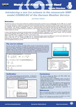
1. QA Tice Sea ice QI Hice Tmelt = -1.7oC The sea ice surface temperature Tice is computed as Ocean with If Tice = 0oC and QA≥ 0 W m-2the sea ice thickness Hice is In all other cases Hice evolves like Synop verification of 2-m temperature [K] in the Baltic Sea domain (s. area indicated in figure left). The experiment ICE is indicated by the red line, REF by the blue line. Figure 1 shows the RMSE against forecast hour for February 2010, 00 UTC runs. In ICE it is reduced by more than 12%. The positive temperature bias is reduced by up to 0.4 K (Fig. 2). Figure 3 shows a negative temperature bias during daytime in April, it is slightly reduced in ICE. Fig. 1: RMSE in Feb. 2010 Fig. 2: Bias in Feb. 2010 Verification domain: Baltic Sea ICE REF Bias RMSE Fig. 3: Bias in Apr. 2010 TEMP verification of air temperature [K] for Tallin, Estonia (26038). The figure shows bias and RMSE for February 2010, 00 UTC runs. In ICE the positive bias of near surface temperature is reduced by up to 0.5 K (after 48h), the RMSE is slightly reduced as well. Introducing a sea ice scheme in the mesoscale NWP model COSMO-EU of the German Weather Service Jan-Peter Schulz Motivation The presence of sea ice on the ocean’s surface has a significant impact on the air-sea interactions. Compared to an open water surface the sea ice completely changes the surface characteristics in terms of albedo and roughness, and therefore substantially changes the surface radiative balance and the turbulent exchange of momentum, heat and moisture between air and sea. In order to deal with these processes the operational global model GME at the German Weather Service (DWD) includes a sea ice scheme (Mironov and Ritter 2004). In contrast, there was no such scheme in DWD’s limited area model COSMO-EU, covering almost all Europe using a mesh size of 7 km. Instead, the GME sea ice surface temperature was interpolated to the COSMO-EU grid at water points which are regarded as being ice covered. This procedure has the disadvantage that the GME sea ice surface temperature is transferred to COSMO-EU only once per day at 00 UTC, as part of the sea surface temperature (SST) analysis, and is then kept constant at this night time value during the data assimilation cycle and also during the forecasts. This means that there is no diurnal cycle of sea ice surface temperature possible in COSMO-EU. Furthermore, the ice temperature of GME may not fit well to the COSMO-EU surface conditions, depending on the weather situation, and may therefore introduce imbalances and noise. For these reasons the GME sea ice scheme was implemented in the COSMO model (cf. Schulz 2011). The sea ice scheme The sea ice scheme by Mironov and Ritter (2004) accounts for thermodynamic processes, while no rheology is considered. It computes the energy balance at the ice’s surface using one layer of ice (s. sketch). This allows for a thermodynamically coupled treatment of sea ice in the COSMO model as lower boundary condition for the atmosphere. In particular, the scheme now allows for a diurnal cycle of sea ice surface temperature. The spatial distribution of sea ice is governed by the data assimilation, the sea ice scheme can not create new ice points by itself. Symbols QA : Total atmospheric energy flux at the ice’s surface QI : Conductive heat flux through the ice layer rice = 910 kg m-3 : Ice density Cice = 2100 J kg-1 K-1 : Ice heat capacity lice = 2.3 W m-1 K-1 : Ice heat conductivity Tbot = -1.7oC : Ice bottom temperature Lf = 0.334 · 106 J kg-1 : Latent heat of freezing c = 0.5 : Shape factor t : Time Verification Conclusions • The sea ice scheme by Mironov and Ritter (2004) was implemented in the COSMO model. • It was successfully tested in COSMO-EU, almost a full cycle of freezing and melting of sea ice in the Baltic Sea from February until May 2010 was simulated. • Verifications for February show significant model improvements in terms of near surface temperature (bias and RMSE) and humidity (not shown), for April there are slight improvements. • The sea ice scheme was operationally implemented in COSMO-EU on 02 Feb. 2011. Two numerical experiments for the period 03 Feb. – 31 May 2010 were carried out with COSMO-EU: one with the sea ice scheme (called ICE) and one without (called REF). References Mironov, D. and B. Ritter, 2004: Testing the new ice model for the global NWP system GME of the German Weather Service; In: J. Cote (Ed.), Research Activities in Atmospheric and Oceanic Modelling, Rep. 34, WMO/TD 1220, WMO, Geneve, 4.21-4.22. Schulz, J.-P., 2011: Introducing a sea ice scheme in the COSMO model, COSMO Newsletter, 11, 32 - 40. (Available at: http://www.cosmo-model.org). Jan-Peter.Schulz@dwd.de Deutscher Wetterdienst http://www.dwd.de