Fields Institute Talk
Fields Institute Talk. Note first half of talk consists of blackboard see video : http ://www.fields.utoronto.ca/video-archive/2013/07/215- 1962 then I did a matlab demo t=1000000; i = sqrt (-1);figure(1);hold off for p=10.^[-3:.2:3 ] % Florent's two coin tosses

Fields Institute Talk
E N D
Presentation Transcript
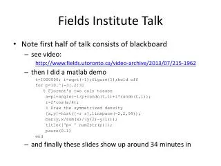
Fields Institute Talk • Note first half of talk consists of blackboard • see video: http://www.fields.utoronto.ca/video-archive/2013/07/215-1962 • then I did a matlab demo t=1000000; i=sqrt(-1);figure(1);hold off for p=10.^[-3:.2:3] % Florent's two coin tosses a=pi+angle(-1/p+randn(t,1)+i*randn(t,1)); r=2*cos(a/4); % Draw the symmetrized density [x,y]=hist([-r r],linspace(-2,2,99)); bar(y,x/sum(x)/(y(2)-y(1))); title(['p= ' num2str(p)]); pause(0.1) end • and finally these slides show up around 34 minutes in
Example Resultp=1 classical probabilityp=0 isotropic convolution (finite free probability) • We call this “isotropic • entanglement”
Preview to the Quantum Information Problem mxmnxn mxmnxn Summands commute, eigenvalues add If A and B are random eigenvalues are classical sum of random variables
Closer to the true problem d2xd2dxd dxd d2xd2 Nothing commutes, eigenvalues non-trivial
Actual Problem di-1xdi-1 d2xd2 dN-i-1xdN-i-1 The Random matrix could be Wishart, Gaussian Ensemble, etc (IndHaar Eigenvectors) The big matrix is dNxdN Interesting Quantum Many Body System Phenomena tied to this overlap!
Intuition on the eigenvectors Classical Quantum Isotropic Intertwined Kronecker Product of Haar Measures
Example Resultp=1 classical convolutionp=0 isotropic convolution
First three moments match theorem • It is well known that the first three free cumulants match the first three classical cumulants • Hence the first three moments for classical and free match • The quantum information problem enjoys the same matching! • Three curves have the same mean, the same variance, the same skewness! • Different kurtoses (4thcumulant/var2+3)
Fitting the fourth moment • Simple idea • Worked better than we expected • Underlying mathematics guarantees more than you would expect • Better approximation • Guarantee of a convex combination between classical and iso
The ProblemLet H= di-1xdi-1 d2xd2 dN-i-1xdN-i-1 Compute or approximate
The ProblemLet H= di-1 d2 dN-i-1 The Random matrix has known joint eigenvalue density & independent eigenvectors distributed with β-Haar measure . β=1 random orthogonal matrix β=2 random unitary matrix β=4 random symplectic matrix General β: formal ghost matrix
Easy Step H= = (odd terms i=1,3,…) + (even terms i=2,4,…) Eigenvalues of odd (even) terms add = Classical convolution of probability densities (Technical note: joint densities needed to preserve all the information) Eigenvectors “fill” the proper slots
Eigenvectors of odd (even) Odd Even Quantify how we are in between Q=I and the full Haar measure
The convolutions • Assume A,B diagonal. Symmetrized ordering. A+B: • A+Q’BQ: • A+Qq’BQq (“hats” indicate joint density is being used)
The Istropically Entangled Approximation The kurtosis But this one is hard
The Slider Theorem p only depends on the eigenvectors! Not the eigenvalues
p vs. Nlarge N: central limit theorem large d, small N: free or isowhole 1 parameter family in between The real world? Falls on a 1 parameter family