Download
1 / 38
520 likes | 838 Vues
ICA and PCA. 學生:周節 教授:王聖智 教授. Outline. Introduction PCA ICA Reference. Introduction. Why are these methods ? A: For computational and conceptual simplicity. And it is more convenient to analysis. What are these methods ?

E N D
ICA and PCA 學生:周節 教授:王聖智 教授
Outline • Introduction • PCA • ICA • Reference
Introduction • Why are these methods ? A: For computational and conceptual simplicity. And it is more convenient to analysis. • What are these methods ? A: The “representation” is often sought as a linear transformation of the original data. • Well-known linear transformation methods. Ex: PCA , ICA , factor analysis, projection pursuit………….
What is PCA? • Principal Component Analysis • It is a way of identifying patterns in data, and expressing the data in such a way as to highlight their similarities and differences. • Reducing the number of dimensions
example • Original data • X Y • 2.5000 2.4000 • 0.5000 0.7000 • 2.2000 2.9000 • 1.9000 2.2000 • 3.1000 3.0000 • 2.3000 2.7000 • 2.0000 1.6000 • 1.0000 1.1000 • 1.5000 1.6000 • 1.1000 0.9000
example (1)Get some data and subtract the mean • X Y • 0.6900 0.4900 • -1.3100 -1.2100 • 0.3900 0.9900 • 0.0900 0.2900 • 1.2900 1.0900 • 0.4900 0.7900 • 0.1900 -0.3100 • -0.8100 -0.8100 • -0.3100 -0.3100 • -0.7100 -1.0100
example (2)Get the covariance matrix Covariance= (3)Get their eigenvectors &eigenvalues 0.6166 0.6154 0.6154 0.7166 eigenvectors = -0.7352 0.6779 0.6779 0.7352 eigenvalues = 0.0491 0 0 1.2840
example eigenvectors -0.7352 0.6779 0.6779 0.7352
Example • (4)Choosing components and forming a feature vector A B eigenvectors -0.7352 0.6779 0.6779 0.7352 eigenvalues 0.0491 0 0 1.2840 B is bigger!
Example • Then we choose two feature vector sets: (a) A+B -0.7352 0.6779 0.6779 0.7352 ( feature vector_1) (b) Only B(Principal Component ) 0.6779 0.7352 ( feature vector_2 ) • Modified_data = feature_vector * old_data
example (a)feature vector_1 • X Y • -0.1751 0.8280 • 0.1429 -1.7776 • 0.3844 0.9922 • 0.1304 0.2742 • -0.2095 1.6758 • 0.1753 0.9129 • -0.3498 -0.0991 • 0.0464 -1.1446 • 0.0178 -0.4380 • -0.1627 -1.2238
example (b)feature vector_2 • x • 0.8280 • -1.7776 • 0.9922 • 0.2742 • 1.6758 • 0.9129 • -0.0991 • -1.1446 • -0.4380 • -1.2238
Example • (5)Deriving the new data set from feature vector (a)feature vector_1 (b)feature vector_2 • New_data = feature_vector_transpose * Modified_data
example (a)feature vector_1 • X Y • 0.6900 0.4900 • -1.3100 -1.2100 • 0.3900 0.9900 • 0.0900 0.2900 • 1.2900 1.0900 • 0.4900 0.7900 • 0.1900 -0.3100 • -0.8100 -0.8100 • -0.3100 -0.3100 • -0.7100 -1.0100
example (b)feature vector_2 • X Y • 0.5613 0.6087 • -1.2050 -1.3068 • 0.6726 0.7294 • 0.1859 0.2016 • 1.1360 1.2320 • 0.6189 0.6712 • -0.0672 -0.0729 • -0.7759 -0.8415 • -0.2969 -0.3220 • -0.8296 -0.8997
Sum Up • 可以降低資料維度 • 資料要有相關性比較適合使用 • 幾何意義:投影到主向量上
What is ICA? • Independent Component Analysis • For separating the blind or unknownsources • Start with “A cocktail-party problem”
ICA • The Principle of ICA: A cocktail-party problem x1(t)=a11 s1(t)+a12 s2(t)+a13 s3(t) x2(t)=a21 s1(t)+a22 s2(t) +a12 s3(t) x3(t)=a31 s1(t)+a32 s2(t) +a33 s3(t)
ICA S1 S2 S3 X1 X2 X3 Linear Transformation
Math model • Given x1(t),x2(t),x3(t) • Want to find s1(t) , s2(t), s3(t) x1(t)=a11 s1(t)+a12 s2(t)+a13 s3(t) x2(t)=a21 s1(t)+a22 s2(t) +a12 s3(t) x3(t)=a31 s1(t)+a32 s2(t) +a33 s3(t) <=>X=AS
Math model X=AS • Because A,S are Unknown • We need some assumption (1) S is statistical independent (2) S is nongaussian distributions • Goal : Find a W such that S=WX
Theorem • Using Central limit theorem The distribution of a sum of independent random variables tends toward a Gaussian distribution Sn Observed signal = a1 S1 + a2 S2 ….+ an toward Gaussian Non-Gaussian Non-Gaussian Non-Gaussian
Theorem • Given x = As Let y = wTx z = ATw => y = wTAs = zTs Xn Observed signal = w1 X1 + w2 X2 ….+ wn Sn = z1 S1 + z2 S2 ….+ zn toward Gaussian Non-Gaussian Non-Gaussian Non-Gaussian
Theorem • Find a w such that Maximization of NonGaussianity of y = wTx • But how to measure NonGaussianity ? Xn Y = w1 X1 + w2 X2 ….+ wn
Theorem • Measures of nongaussianity • Kurtosis: • As y toward to gaussian , F(y) is much closer to zero !!! F(y) = E{ (y)4 } - 3*[ E{ (y)2 } ] 2 Super-Gaussian kurtosis > 0 Gaussian kurtosis = 0 Sub-Gaussian kurtosis < 0
Steps • (1) centering & whitening process • (2) FastICA algorithm
Steps Linear Transformation X1 X2 X3 S1 S2 S3 centering & whitening Z1 Z2 Z3 FastICA X1 X2 X3 S1 S2 S3 Correlated uncorrelated independent
example • Original data
example • (1) centering & whitening process
example (2) FastICA algorithm
example (2) FastICA algorithm
Sum up • 能讓成份間的統計相關性(statistical dependent)達到最小的線性轉換方法 • 可以解決未知訊號分解的問題( Blind Source Separation )
Reference • “A tutorial on Principal Components Analysis”, Lindsay I Smith , February 26, 2002 • “Independent Component Analysis : Algorithms and Applications “, Aapo Hyvärinen and Erkki Oja , Neural Networks Research Centre Helsinki University of Technology • http://www.cis.hut.fi/projects/ica/icademo/
1 - = = T z Vx D E x 2 centering & Whitening process = is zero mean x A s • Let • Let D and E be the eigenvalues and eigenvector matrix of • covariance matrix of x, i.e. = T T E { xx } EDE 1 - • Then is a whitening matrix = T V D E 2 = T T T E { zz } V E { xx } V 1 1 - - = T T D E EDE ED 2 2 = I
centering & Whitening process For the whitened data z, find a vector w such that the linear combination y=wTz has maximum nongaussianity under the constrain Then Maximize | kurt(wTz)| under the simpler constraint that ||w||=1
FastICA • Centering • Whitening • Choose m, No. of ICs to estimate. Set counter p 1 • Choose an initial guess of unit norm for wp, eg. randomly. • Let • Do deflation decorrelation • Let wp wp/||wp|| • If wp has not converged (|<wpk+1 , wpk>| 1), go to step 5. • Set p p+1. If p m, go back to step 4.