PCA

1. PCA Mechanics

2. Component • The component is a linear combination of the original variables • The variance of y1 is maximized subject to the constraint that the sum of the squared weights equals 1 • Using standardized data • The second component is conducted in the same manner with the additional restraint that it has zero correlation with the first component • Together the two components would have the highest possible sum of squared multiple correlations with the original variables

3. Variance • The variance of a linear composite • Is • Where σij is the covariance between the variables in question • The matrix formulation involves pre and post multiplying the covariance matrix C by the vector of weights

4. Variance • PCA finds the vector of weights (a) that maximizes • Such that

5. Variance • The variance of the component (eigenvalue) will be labeled as λ • The sum of the λs is equal to the sum of the variances of the original variables • If the variables are standardized, the sum equals the number of variables, and dividing the eigenvalue by the number of variables gives us an ‘amount of variance accounted for’ by that component

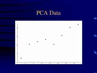
6. Data height weight Zheight Zweight 57 93 -1.77427146053986 -1.96516286068824 58 110 -1.47097719378091 -.873405715861441 60 99 -.86438866026301 -1.5798368095729 59 111 -1.16768292702196 -.809184707342218 61 115 -.561094393504058 -.552300673265324 60 122 -.86438866026301 -.102753613630758 62 110 -.257800126745107 -.873405715861441 61 116 -.561094393504058 -.4880796647461 62 122 -.257800126745107 -.102753613630758 63 128 .0454941400138444 .282572437484583 62 134 -.257800126745107 .667898488599925 64 117 .348788406772796 -.423858656226876 63 123 .0454941400138444 -.0385326051115347 65 129 .652082673531747 .346793446003807 64 135 .348788406772796 .732119497119148 66 128 .955376940290699 .282572437484583 67 135 1.25867120704965 .732119497119148 66 148 .955376940290699 1.56699260786906 68 142 1.5619654738086 1.18166655675371 69 155 1.86525974056755 2.01653966750362 Example data of women’s height and weight

7. Geometric view • This graph shows the relationship of two standardized variables, height and weight • As such, the 0,0 origin represents their means • With two standardized variables, we’d have two weights to use in creation of the linear combination • And they’d be .707,.707 for the first component which is always at a 450 angle when dealing with 2 variables • Cosine of 450 is .707 • .707*(-.86)+.707*(-.10) = -.68 • The projection of a point on a coordinate axis is the numerical value on the coordinate axis at which a line from the original point drawn perpendicular to the axis intersects the axis

8. Geometric view • The second component captures the remaining variance, and is uncorrelated to the first • Cosine of the angle formed by the two axes (900) is zero • Note that with Factor analysis we may want to examine correlated factors, and so the axes regarding their components would be allowed not to be perpendicular

9. Geometric view • The other eigenvector associated with the data is (-.707,.707) • Doing as we did before we’d create that second axis, and then could plot the data points along these new axes as in the figure • We now have two linear combinations, each of which is interpretable as the vector whose components are projections of points onto a directed line segment • Note how the basic shape of the original data has been perfectly maintained • The effect has been to rotate the configuration (45o) to a new orientation while preserving its essential size and shape • It is an orthogonal rotation

10. Rotation • Sometimes the loadings will not be easily interpretable in PCA • One way to help is to rotate the axes in that geometric space, and a rotation that maintains the independence of the components may be useful in this regard • We take the factor loading matrix and multiply it by a transformation matrix to produce a new, rotated loading matrix

11. Rotation • Consider the varimax rotation • It finds a rotation matrix (Λ) that will result in transformed loadings in which the high loadings will become higher, and low loadings lower • An example with four variables, looking at the first two components

12. Rotation • What we have done is rotate the axes 190 • The transformation matrix corresponds to the following • Ψ is the angle of rotation More will be discussed regarding rotation when we get into Factor analysis

13. Stretching and shrinking • Note that with what we have now there are two new variables, Z1 and Z2, with very different variances • Z1 much larger • If we want them to be equal we can simply standardize those Z1 and Z2 values • s2 = 1 for both • In general, multiplying a matrix by a scalar will shrink or stretch the plot • Here, let Z be the matrix of the Z variables and D a diagonal matrix with the standard deviations on the diagonal • The resulting plot would now be circular

14. Singular value decomposition • Given a data matrix X, we can use one matrix operation to stretch or shrink the values • Multiply by a scalar • < 1 shrink • > 1 stretch • We’ve just seen how to rotate the values • Matrix multiplication • In general we can start with a matrix X and get • Zs = X W D-1 • W here is the matrix that specifies the rotation by some amount (degrees) • With a little reworking • X = Zs DW’ • What this means is that any data matrix X can be decomposed into three parts: • A matrix of uncorrelated variables with variance/sd = 1 (Zs) • A stretching and shrinking transformation (D) • And an orthogonal rotation (W’) • Finding these components is called singular value decomposition

15. The Determinant • The determinant of a var/covar matrix provides a single measure of the variance in the variables • Generalized variance • 10.87*224.42 – 44.51*44.51 = 654 • Note • 44.51/√(10.87*224.42) = r = .867 VarCovar matrix for the data 10.87 44.51 44.51 224.42

16. Geometric interpretation of the determinant • Suppose we use the values from our variance/covariance matrix and plot them geometrically as coordinates • The vectors emanating from the origin to those points defines a parrallelogram • In general the skinnier the parallelogram, the larger the correlation • Here ours is pretty skinny due to an r = .867 • The determinant is the area of this parallelogram, and thus will be smaller with larger correlations • Recall our collinearity problem • The top is that associated with the raw variables varcovar matrix • The bottom is that of the components Z1 and Z2

17. The scatterplots illustrate two variables with increasing correlations 0,.25,.50,.75,1. • The smaller plots are the plot of the correlation matrix in 2d space (e.g. the coordinates for the 4th diagram are 1, .75 for one point, .75,1 for the other). • The eigenvalues associated with the correlation matrix are the lengths of the major and minor axes, e.g. 1.75 and .25 for diagram 4. • Also drawn is the ellipse specified by the axes

18. Summary • We can think of PCA as a data reduction technique • Although it will produce as many components as variables, we will only be interested in those which account for at least as much variance as a variable (i.e. eigenvalue of 1 or greater) • We are interested in how many components are retained and their interpretation • Furthermore, if interpretability of the loadings is not straightforward, we can rotate the solution for a better understanding