PCA + SVD
PCA + SVD. Motivation – Shape Matching. There are tagged feature points in both sets that are matched by the user. What is the best transformation that aligns the unicorn with the lion?. Motivation – Shape Matching. Regard the shapes as sets of points and try to “match” these sets

PCA + SVD
E N D
Presentation Transcript
Motivation – Shape Matching There are tagged feature points in both sets that are matched by the user What is the best transformation that aligns the unicorn with the lion?
Motivation – Shape Matching Regard the shapes as sets of points and try to “match” these sets using a linear transformation The above is not a good alignment….
Motivation – Shape Matching • Alignment by translation or rotation • The structure stays “rigid” under these two transformations • Called rigid-body or isometric (distance-preserving)transformations • Mathematically, they are represented as matrix/vector operations Before alignment After alignment
Transformation Math y • Translation • Vector addition: • Rotation • Matrix product: x
Alignment • Input: two models represented as point sets • Source and target • Output: locations of the translated and rotated source points Source Target
Alignment • Method 1: Principal component analysis (PCA) • Aligning principal directions • Method 2: Singular value decomposition (SVD) • Optimal alignment given prior knowledge of correspondence • Method 3: Iterative closest point (ICP) • An iterative SVD algorithm that computes correspondences as it goes
Method 1: PCA • Compute a shape-aware coordinate system for each model • Origin: Centroid of all points • Axes: Directions in which the model varies most or least • Transform the source to align its origin/axes with the target
Method 1: PCA • Computing axes: Principal Component Analysis (PCA) • Consider a set of points p1,…,pn with centroid location c • Construct matrix P whose i-thcolumn is vector pi – c • 2D (2 by n): • 3D (3 by n): • Build the covariance matrix: • 2D: a 2 by 2 matrix • 3D: a 3 by 3 matrix
Method 1: PCA • Computing axes: Principal Component Analysis (PCA) • Eigenvectors of the covariance matrix represent principal directions of shape variation (2 in 2D; 3 in 3D) • The eigenvectors are orthogonal, and have no magnitude; only directions • Eigenvalues indicate amount of variation along each eigenvector • Eigenvector with largest (smallest) eigenvalue is the direction where the model shape varies the most (least) Eigenvector with the smallest eigenvalue Eigenvector with the largest eigenvalue
2nd (right) singular vector 1st (right) singular vector: direction of maximal variance, 2nd (right) singular vector: direction of maximal variance, after removing the projection of the data along the first singular vector. 1st (right) singular vector Method 1: PCAWhy do we look at the singular vectors?On the board… Input:2-d dimensional points Output:
Method 1: PCACovariance matrix • Goal: reduce the dimensionality while preserving the “information in the data” • Information in the data: variability in the data • We measure variability using the covariance matrix. • Sample covariance of variables X and Y • Given matrix A, remove the mean of each column from the column vectors to get the centered matrix C • The matrix is the covariance matrix of the row vectors of A.
Method 1: PCA • We will project the rows of matrix A into a new set of attributes (dimensions) such that: • The attributes have zero covariance to each other (they are orthogonal) • Each attribute captures the most remaining variance in the data, while orthogonal to the existing attributes • The first attribute should capture the most variance in the data • For matrix C, the variance of the rows of C when projected to vector x is given by • The right singular vector of C maximizes !
2nd (right) singular vector 1st (right) singular vector: direction of maximal variance, 2nd (right) singular vector: direction of maximal variance, after removing the projection of the data along the first singular vector. 1st (right) singular vector Method 1: PCA Input:2-d dimensional points Output:
2nd (right) singular vector 1st (right) singular vector Method 1: PCASingular values 1: measures how much of the data variance is explained by the first singular vector. 2: measures how much of the data variance is explained by the second singular vector. 1
Method 1: PCASingular values tell us something about the variance • The variance in the direction of the k-th principal component is given by the corresponding singular value σk2 • Singular values can be used to estimate how many components to keep • Rule of thumb: keep enough to explain 85% of the variation:
1st (right) singular vector Method 1: PCA Another property of PCA • The chosen vectors are such that minimize the sum of square differences between the data vectors and the low-dimensional projections
Method 1: PCA • Limitations • Centroid and axes are affected by noise Noise Axes are affected PCA result
Method 1: PCA • Limitations • Axes can be unreliable for circular objects • Eigenvalues become similar, and eigenvectors become unstable PCA result Rotation by a small angle
Method 2: SVD • Optimal alignment between corresponding points • Assuming that for each source point, we know where the corresponding target point is.
Method 2: SVDSingular Value Decomposition [n×m] = [n×r] [r×r] [r×m] r: rank of matrix A U,V are orthogonal matrices
Method 2: SVD • Formulating the problem • Source points p1,…,pn with centroid location cS • Target points q1,…,qn with centroid location cT • qi is the corresponding point of pi • After centroid alignment and rotation by some R, a transformed source point is located at: • We wish to find the R that minimizes sum of pair-wise distances: • Solving the problem – on the board…
Method 2: SVD • SVD-based alignment: summary • Forming the cross-covariance matrix • Computing SVD • The optimal rotation matrix is • Translate and rotate the source: Translate Rotate
Method 2: SVD • Advantage over PCA: more stable • As long as the correspondences are correct
Method 2: SVD • Advantage over PCA: more stable • As long as the correspondences are correct
Method 2: SVD • Limitation: requires accurate correspondences • Which are usually not available
Method 3: ICP • The idea • Use PCA alignment to obtain initial guess of correspondences • Iteratively improve the correspondences after repeated SVD • Iterative closest point (ICP) • 1. Transform the source by PCA-based alignment • 2. For each transformed source point, assign the closest target point as its corresponding point. Align source and target by SVD. • Not all target points need to be used • 3. Repeat step (2) until a termination criteria is met.
ICP Algorithm After PCA After 1 iter After 10 iter
ICP Algorithm After PCA After 1 iter After 10 iter
ICP Algorithm • Termination criteria • A user-given maximum iteration is reached • The improvement of fitting is small • Root Mean Squared Distance (RMSD): • Captures average deviation in all corresponding pairs • Stops the iteration if the difference in RMSD before and after each iteration falls beneath a user-given threshold
More Examples After PCA After ICP