PCA Channel
PCA Channel. Student: Fangming JI u4082259 Supervisor: Professor Tom Geoden. Organization of the Presentation. PCA and problems PCA channel idea Use the channel for automatic classification Channel Corrected Channel Conclusion Future work. Principle Component Analysis. A statistic tool


PCA Channel
E N D
Presentation Transcript
PCA Channel Student: Fangming JI u4082259 Supervisor: Professor Tom Geoden
Organization of the Presentation • PCA and problems • PCA channel idea • Use the channel for automatic classification • Channel • Corrected Channel • Conclusion • Future work
Principle Component Analysis • A statistic tool • Maximizes the scatter of all projected samples in the image space. • Tries to capture the most important features and reduce the dimensions at the same time • Each eigenvector is a principle component
Algorithm of PCA • Given a training set of M images with the same size, convert each of them into a single dimension vector (I1, I2, … Im) Then, find the average image by calculating the mean of the training set Ψ = (∑In) / M, n = 1, …m. Each training image differs from the average by Φn = In - Ψ. Then, the covariance matrix C is found by • where A = [Φ1, Φ2, … Φm] and C is a matrix. It is too big to be used in practice. But fortunately, there are only M-1 non-zero eigenvalues and they can be found more efficiently with an M x M computation. This means that we can compute the eigenvector viof instead of computing the eigenvector ui of . Also we can notice that the M best eigenvalues of are equal to the M best eigenvalues of . Then we can get M best eigenvalues of ui by Avi. At the end we will select a value K, to keep only K largest eigenvalues.
Problems of PCA based methods • Avalanche disaster • Up to a certain limit, these methods are robust over a wide range of parameter. • Algorithm breaks down dramatically beyond that point
Constant Features and Inconstant Features • Holistic features = Local features + inconstant features • Local Features (constant features) • Inconstant features (such as view, illumination and expressions) • Little change from inconstant => Little change for holistic one • Great change of inconstant => maybe great change for the holistic one
Distribution in the Image Space • Images from the same personality may sit in totally different regions of the images space. • Distance between the images beyond the range of being correctly recognized
The PCA Channel • Holistic features = Local features + inconstant features • Positions decided by both local features and inconstant features • Incremental changes in the inconstant features, should produce incremental changed holistic features or positions • This incremental changed position looks like a channel so we call it “PCA Channel”
Experiment Preparation And Tools • Collecting images with incremental changes in the orientations -- Mingtao’s software • 45 images from three identities (15 images for each identity which are changed incrementally in orientation) • Dozens of images from another three identities, randomly oriented with some expression images • Face Recognition Practitioner – Software developed by me
Existence of The Channel • Take view for example
1)Given an input image 2)Recognize it 3) Compute the PCA again with the new recognized image 4) Go to step 1) 1) Give an input image 2) Recognize it 3) Put it into the training set 4) Go to step 1) Automatic Image Classification • Original PCA method • The PCA channel method
Performance Comparison • If the training set is carefully selected the performance of PCA channel is better than the original one • Problems: • Sensitive to the selection of the training set • Contagious problem
The Corrected PCA Channel • Cut off the root of the mismatching • Improve the robustness
Implementation • Set up two threshold: Low(L) and High(H) • If the distance between the input image and the its nearest image in the training set < L, recognize it. If the distance > H, put it for future recognition; if L < distance < H, make it a new group. • Calculate the PCA again and cut off the mismatching at here • Match again
Results • The success rate = Match to Original Training Set + Match to New Group • The success rate = 44.15%+50.65% = 94.80% • The success rate = 44.15%+51.94% = 96.09% • 59.74%
Conclusion • Properly build up image database and the PCA channel with cautious implementation, we can get very good performance for face recognition. • But from the above experiment we can see that, the strength but also the weakness of the PCA channel is the images database. • 3D face reconstruction system. • Large computational load. But it can also be appropriate in some situations where the focus is more on accuracy than response time.
Future Works • Verify Our Research On Larger Data Set • Preprocess the images before recognition • Build Up a 3D-Face Morphable Model System • Research in Hybrid Methods