Download
1 / 18
180 likes | 341 Vues
A spectral finite volume transport scheme on the cubed-sphere. Vani Cheruvu, Ramachandran D. Nair, Henry M. Tufo Department of Computer Science, University of Colorado at Boulder, Boulder, CO 80309, USA

E N D
A spectral finite volume transport scheme on the cubed-sphere Vani Cheruvu, Ramachandran D. Nair, Henry M. Tufo Department of Computer Science, University of Colorado at Boulder, Boulder, CO 80309, USA Scientific Computing Division, National Center for Atmospheric Research, Boulder, CO 80305, USA Presented by Kiran Katta
Overview Advection, role in Atmospheric Dynamics. Properties of numerical schemes required. The Spectral Finite Volume(SFV) method. SFV method in two dimensions. Numerical example, the spectral accuracy of the proposed SFV scheme. Application of the SFV scheme on the cubed-sphere. Summary and Conclusions.
Advective Process Crucial in Numerical Modeling. Accurately capturing these Advective Processes.
Numerical scheme's properties Monotonicity. Small Numerical Diffusion. Mass Conservation. High Accuracy. Reasonable Computational Cost.
Spectral Finite Volume(SFV) Method Evolution Global Spectral Transform Methods used before Spectral Element Method. Dis-Advantages: Expensive non-local communication operations. SE Method: Combine the accuracy of conventional spectral methods and the geometric flexibility of finite element methods. Dis-Advantages: Non conservative. Spectral Finite Volume method was proposed with high-order conservation. In this paper, SFV scheme for transport equation was developed.
SFV method in Two Dimensions Two-Dimensional Scalar Conservation Law ∂U/ ∂t + ∇ · F(U ) = 0, in D × (0, T ), ∀(x, y) ∈ D U = U (x, y, t), ∇ ≡ (∂/∂x, ∂/∂y), and Flux fn - F = (F, G) Init Condn: U0 (x, y) = U (x, y, t = 0), D is periodic. SFV formulation: Based on the Classical Finite Volume Method. Ω =UΩCV Ω = Spectral Volume
SFV method in Two Dimensions The finite volume form of the transport equation for ΩCV: Where Nf is the # of faces in ΩCV, Γr is the rth face, Acv is the area of ΩCV Numerical approx: evaluating the boundary integral and in time-stepping the cell averages.
Spatial Discretization for Rectangular Elements D be partitioned into Nx X Ny rectangular elements. Dpq = (x, y) | x ∈ [xp−1/2, xp+1/2], y ∈ [yq−1/2, yq+1/2] Interpolation points to be Gauss–Lobatto–Legendre (GLL) point. An approx sol UΩ in any SV Ω is: Ulm are fn values at GLL pts on Ω. The nodal basis set is made using Lagrange–Legendre polynomials with roots at GLL pts. Lk(ξ ) is the Legendre polynomial of deg k, ξ is (k + 1) GLL roots.
High-order reconstruction for SFV Finding the cell-edge values. Reconstruction for the SFV method based on an accumulated mass approach. Accumulated mass Density ρ(ξ) at the cell edge This can be extended to 2D by a tensor-product of 1D operations Acc masses are estimated at CV boundaries Differentiation is applied to get intermediate edge values. Accumulated mass is computed from these.
Flux evaluation Evaluate the fluxes at the CV boundaries. The flux values are not uniquely defined. The analytic flux is replaced by a numerical flux by solving a Riemann problem. Local Lax–Friedrichs flux formula α is the local upper bound on |F’(U)|
Time Integration Strong stability preserving 3-order Runge–Kutta time discretization is used. Flux-corrected Transport Algorithm The FCT algorithm requires the calculation of two sets of fluxes. The main steps in the SFV-FCT algorithm for the transport model are 1.Compute the cell averages (U¯)^n for the initial condition. 2. Compute the monotonic upwind fluxes. 3. Advance the cell averages in time to obtain the diffusive sol. 4. Compute the high-order fluxes corresp to the SFV scheme. 5. Compute the anti-diffusive fluxes. 6. advance the cell averages based on the limited anti-diffusive fluxes.
Numerical experiments Spectral accuracy of the proposed SFV scheme for a smooth problem to verify correctness Demonstration of spectral accuracy with linear wave equation (a) fixed element partition: N number of elements with varying order of accuracy (b) fixed order of accuracy: k number of cells with varying number of elements.
Numerical Tests Solid body rotation of a non-smooth function. Contour lines of the solid-body rotation of the function given after 1/4th of the rotation. Left panel shows the solution using the SFV scheme and the right panel shows the solution using the SFV-FCT scheme
Numerical Tests Deformational flow Left panel shows the exact solution and the right panel shows the computed solution
Application of the SFV scheme on the cubed-sphere To avoid singularities at the poles cubed-sphere geometry is used. v = u1a1 + u2a2 Transform spherical velocity to cubed sphere Velocity vectors Where A and A−1 are “cube-to-sphere” and the “sphere-to-cube” transformation matrices. The metric tensor is For SFV, the total # of SVs on cubed sphere is 6 x N2e and CVs is 6 x N2e x k2.
Conservative Transport on Cubed-Sphere The continuity equation in flux form, on the sphere φ is the advecting field and v = v(λ, θ) is the horizontal wind vector
Numerical experiments Perform standard advection tests, known as solid-body rotation. The initial scalar field is defined as The left panel shows the cosine bell at the initial pt. The right panel displays solution at the first vertex. The cosine bell smoothly crosses over the corner point.