CSE332: Data Abstractions Lecture 11: Hash Tables
530 likes | 711 Vues
CSE332: Data Abstractions Lecture 11: Hash Tables. Dan Grossman Spring 2012. Hash Tables: Review. Aim for constant-time (i.e., O (1)) find , insert , and delete “On average” under some reasonable assumptions A hash table is an array of some fixed size But growable as we’ll see.

CSE332: Data Abstractions Lecture 11: Hash Tables
E N D
Presentation Transcript
CSE332: Data AbstractionsLecture 11: Hash Tables Dan Grossman Spring 2012
Hash Tables: Review • Aim for constant-time (i.e., O(1)) find, insert, and delete • “On average” under some reasonable assumptions • A hash table is an array of some fixed size • But growable as we’ll see hash table hash table library client collision? collision resolution int table-index E TableSize –1 CSE332: Data Abstractions
Collision resolution Collision: When two keys map to the same location in the hash table We try to avoid it, but number-of-keys exceeds table size So hash tables should support collision resolution • Ideas? CSE332: Data Abstractions
Separate Chaining Chaining: All keys that map to the same table location are kept in a list (a.k.a. a “chain” or “bucket”) As easy as it sounds Example: insert 10, 22, 107, 12, 42 with mod hashing and TableSize = 10 CSE332: Data Abstractions
Separate Chaining 10 / Chaining: All keys that map to the same table location are kept in a list (a.k.a. a “chain” or “bucket”) As easy as it sounds Example: insert 10, 22, 107, 12, 42 with mod hashing and TableSize = 10 CSE332: Data Abstractions
Separate Chaining 10 / Chaining: All keys that map to the same table location are kept in a list (a.k.a. a “chain” or “bucket”) As easy as it sounds Example: insert 10, 22, 107, 12, 42 with mod hashing and TableSize = 10 22 / CSE332: Data Abstractions
Separate Chaining 10 / Chaining: All keys that map to the same table location are kept in a list (a.k.a. a “chain” or “bucket”) As easy as it sounds Example: insert 10, 22, 107, 12, 42 with mod hashing and TableSize = 10 22 / 107 / CSE332: Data Abstractions
Separate Chaining 10 / Chaining: All keys that map to the same table location are kept in a list (a.k.a. a “chain” or “bucket”) As easy as it sounds Example: insert 10, 22, 107, 12, 42 with mod hashing and TableSize = 10 12 22 / 107 / CSE332: Data Abstractions
Separate Chaining 10 / Chaining: All keys that map to the same table location are kept in a list (a.k.a. a “chain” or “bucket”) As easy as it sounds Example: insert 10, 22, 107, 12, 42 with mod hashing and TableSize = 10 42 12 22 / 107 / CSE332: Data Abstractions
Thoughts on chaining • Worst-case time for find? • Linear • But only with really bad luck or bad hash function • So not worth avoiding (e.g., with balanced trees at each bucket) • Beyond asymptotic complexity, some “data-structure engineering” may be warranted • Linked list vs. array vs. chunked list (lists should be short!) • Move-to-front (cf. Project 2) • Better idea: Leave room for 1 element (or 2?) in the table itself, to optimize constant factors for the common case • A time-space trade-off… CSE332: Data Abstractions
Time vs. space (constant factors only here) 10 / 12 22 / 42 12 22 / 107 / CSE332: Data Abstractions
More Rigorous Chaining Analysis Definition: The load factor, , of a hash table is number of elements • Under chaining, the average number of elements per bucket is ____ • So if some inserts are followed by random finds, then on average: • Each unsuccessful find compares against ____ items • Each successful find compares against _____ items CSE332: Data Abstractions
More rigorous chaining analysis Definition: The load factor, , of a hash table is number of elements • Under chaining, the average number of elements per bucket is • So if some inserts are followed by random finds, then on average: • Each unsuccessful find compares against items • Each successful find compares against / 2 items • So we like to keep fairly low (e.g., 1 or 1.5 or 2) for chaining CSE332: Data Abstractions
Alternative: Use empty space in the table • Another simple idea: If h(key) is already full, • try (h(key) + 1) % TableSize. If full, • try (h(key) + 2) % TableSize. If full, • try (h(key) + 3) % TableSize. If full… • Example: insert 38, 19, 8, 109, 10 CSE332: Data Abstractions
Alternative: Use empty space in the table • Another simple idea: If h(key) is already full, • try (h(key) + 1) % TableSize. If full, • try (h(key) + 2) % TableSize. If full, • try (h(key) + 3) % TableSize. If full… • Example: insert 38, 19, 8, 109, 10 CSE332: Data Abstractions
Alternative: Use empty space in the table • Another simple idea: If h(key) is already full, • try (h(key) + 1) % TableSize. If full, • try (h(key) + 2) % TableSize. If full, • try (h(key) + 3) % TableSize. If full… • Example: insert 38, 19, 8, 109, 10 CSE332: Data Abstractions
Alternative: Use empty space in the table • Another simple idea: If h(key) is already full, • try (h(key) + 1) % TableSize. If full, • try (h(key) + 2) % TableSize. If full, • try (h(key) + 3) % TableSize. If full… • Example: insert 38, 19, 8, 109, 10 CSE332: Data Abstractions
Alternative: Use empty space in the table • Another simple idea: If h(key) is already full, • try (h(key) + 1) % TableSize. If full, • try (h(key) + 2) % TableSize. If full, • try (h(key) + 3) % TableSize. If full… • Example: insert 38, 19, 8, 109, 10 CSE332: Data Abstractions
Open addressing This is one example of open addressing In general, open addressing means resolving collisions by trying a sequence of other positions in the table. Trying the next spot is called probing • We just did linear probing • ith probe was (h(key) + i) % TableSize • In general have some probe functionf and use h(key) + f(i) % TableSize Open addressing does poorly with high load factor • So want larger tables • Too many probes means no more O(1) CSE332: Data Abstractions
Terminology We and the book use the terms • “chaining” or “separate chaining” • “open addressing” Very confusingly, • “open hashing” is a synonym for “chaining” • “closed hashing” is a synonym for “open addressing” (If it makes you feel any better, most trees in CS grow upside-down ) CSE332: Data Abstractions
Other operations insert finds an open table position using a probe function What about find? • Must use same probe function to “retrace the trail” for the data • Unsuccessful search when reach empty position What about delete? • Must use “lazy” deletion. Why? • Marker indicates “no data here, but don’t stop probing” • Note: delete with chaining is plain-old list-remove CSE332: Data Abstractions
(Primary) Clustering It turns out linear probing is a bad idea, even though the probe function is quick to compute (which is a good thing) Tends to produce clusters, which lead to long probingsequences • Called primary clustering • Saw this starting in our example [R. Sedgewick] CSE332: Data Abstractions
Analysis of Linear Probing • Trivial fact: For any < 1, linear probing will find an empty slot • It is “safe” in this sense: no infinite loop unless table is full • Non-trivial facts we won’t prove: Average # of probes given (in the limit as TableSize → ) • Unsuccessful search: • Successful search: • This is pretty bad: need to leave sufficient empty space in the table to get decent performance (see chart) CSE332: Data Abstractions
In a chart • Linear-probing performance degrades rapidly as table gets full • (Formula assumes “large table” but point remains) • By comparison, chaining performance is linear in and has no trouble with >1 CSE332: Data Abstractions
Quadratic probing • We can avoid primary clustering by changing the probe function (h(key) + f(i)) % TableSize • A common technique is quadratic probing: f(i) = i2 • So probe sequence is: • 0th probe: h(key) % TableSize • 1st probe: (h(key) + 1) % TableSize • 2nd probe: (h(key) + 4) % TableSize • 3rd probe: (h(key) + 9) % TableSize • … • ith probe: (h(key) + i2)% TableSize • Intuition: Probes quickly “leave the neighborhood” CSE332: Data Abstractions
Quadratic Probing Example TableSize=10 Insert: 89 18 49 58 79 CSE332: Data Abstractions
Quadratic Probing Example TableSize=10 Insert: 89 18 49 58 79 CSE332: Data Abstractions
Quadratic Probing Example TableSize=10 Insert: 89 18 49 58 79 CSE332: Data Abstractions
Quadratic Probing Example TableSize=10 Insert: 89 18 49 58 79 CSE332: Data Abstractions
Quadratic Probing Example TableSize=10 Insert: 89 18 49 58 79 CSE332: Data Abstractions
Quadratic Probing Example TableSize=10 Insert: 89 18 49 58 79 CSE332: Data Abstractions
Another Quadratic Probing Example TableSize = 7 Insert: (76 % 7 = 6) (40 % 7 = 5) 48 (48 % 7 = 6) 5 ( 5 % 7 = 5) 55 (55 % 7 = 6) 47 (47 % 7 = 5) CSE332: Data Abstractions
Another Quadratic Probing Example TableSize = 7 Insert: (76 % 7 = 6) (40 % 7 = 5) 48 (48 % 7 = 6) 5 ( 5 % 7 = 5) 55 (55 % 7 = 6) 47 (47 % 7 = 5) CSE332: Data Abstractions
Another Quadratic Probing Example TableSize = 7 Insert: (76 % 7 = 6) (40 % 7 = 5) 48 (48 % 7 = 6) 5 ( 5 % 7 = 5) 55 (55 % 7 = 6) 47 (47 % 7 = 5) CSE332: Data Abstractions
Another Quadratic Probing Example TableSize = 7 Insert: (76 % 7 = 6) (40 % 7 = 5) 48 (48 % 7 = 6) 5 ( 5 % 7 = 5) 55 (55 % 7 = 6) 47 (47 % 7 = 5) CSE332: Data Abstractions
Another Quadratic Probing Example TableSize = 7 Insert: (76 % 7 = 6) (40 % 7 = 5) 48 (48 % 7 = 6) 5 ( 5 % 7 = 5) 55 (55 % 7 = 6) 47 (47 % 7 = 5) CSE332: Data Abstractions
Another Quadratic Probing Example TableSize = 7 Insert: (76 % 7 = 6) (40 % 7 = 5) 48 (48 % 7 = 6) 5 ( 5 % 7 = 5) 55 (55 % 7 = 6) 47 (47 % 7 = 5) CSE332: Data Abstractions
Another Quadratic Probing Example TableSize = 7 Insert: (76 % 7 = 6) (40 % 7 = 5) 48 (48 % 7 = 6) 5 ( 5 % 7 = 5) 55 (55 % 7 = 6) 47 (47 % 7 = 5) • Doh!: For all n, ((n*n) +5) % 7 is 0, 2, 5, or 6 • Excel shows takes “at least” 50 probes and a pattern • Proof uses induction and (n2+5) % 7 = ((n-7)2+5) % 7 • In fact, for all c and k, (n2+c) % k = ((n-k)2+c) % k CSE332: Data Abstractions
From Bad News to Good News • Bad news: • Quadratic probing can cycle through the same full indices, never terminating despite table not being full • Good news: • If TableSize is prime and < ½, then quadratic probing will find an empty slot in at most TableSize/2 probes • So: If you keep < ½ and TableSize is prime, no need to detect cycles • Proof is posted in lecture11.txt • Also, slightly less detailed proof in textbook • Key fact: For prime T and 0 < i,j < T/2 where i j, (k + i2) % T (k + j2) % T (i.e., no index repeat) CSE332: Data Abstractions
Clustering reconsidered • Quadratic probing does not suffer from primary clustering: no problem with keys initially hashing to the same neighborhood • But it’s no help if keys initially hash to the same index • Called secondary clustering • Can avoid secondary clustering with a probe function that depends on the key: double hashing… CSE332: Data Abstractions
Double hashing Idea: • Given two good hash functions h and g, it is very unlikely that for some key, h(key) == g(key) • So make the probe function f(i) = i*g(key) Probe sequence: • 0th probe: h(key) % TableSize • 1st probe: (h(key) + g(key)) % TableSize • 2nd probe: (h(key) + 2*g(key)) % TableSize • 3rd probe: (h(key) + 3*g(key)) % TableSize • … • ith probe: (h(key) + i*g(key))% TableSize Detail: Make sure g(key) cannot be 0 CSE332: Data Abstractions
Double-hashing analysis • Intuition: Because each probe is “jumping” by g(key) each time, we “leave the neighborhood” and “go different places from other initial collisions” • But we could still have a problem like in quadratic probing where we are not “safe” (infinite loop despite room in table) • It is known that this cannot happen in at least one case: • h(key) = key % p • g(key) = q – (key % q) • 2 < q < p • p and q are prime CSE332: Data Abstractions
More double-hashing facts • Assume “uniform hashing” • Means probability of g(key1) % p == g(key2) % p is 1/p • Non-trivial facts we won’t prove: Average # of probes given (in the limit as TableSize → ) • Unsuccessful search (intuitive): • Successful search (less intuitive): • Bottom line: unsuccessful bad (but not as bad as linear probing), but successful is not nearly as bad CSE332: Data Abstractions
Charts CSE332: Data Abstractions
Where are we? • Chaining is easy • find, delete proportional to load factor on average • insert can be constant if just push on front of list • Open addressing uses probing, has clustering issues as table fills • Why use it: • Less memory allocation? • Easier data representation? • Now: • Growing the table when it gets too full (“rehashing”) • Relation between hashing/comparing and connection to Java CSE332: Data Abstractions
Rehashing • As with array-based stacks/queues/lists, if table gets too full, create a bigger table and copy everything • With chaining, we get to decide what “too full” means • Keep load factor reasonable (e.g., < 1)? • Consider average or max size of non-empty chains? • For open addressing, half-full is a good rule of thumb • New table size • Twice-as-big is a good idea, except, uhm, that won’t be prime! • So go about twice-as-big • Can have a list of prime numbers in your code since you won’t grow more than 20-30 times CSE332: Data Abstractions
More on rehashing • What if we copy all data to the same indices in the new table? • Will not work; we calculated the index based on TableSize • Go through table, do standard insert for each into new table • Run-time? • O(n): Iterate through old table • Resize is an O(n) operation, involving n calls to the hash function • Is there some way to avoid all those hash function calls? • Space/time tradeoff: Could store h(key) with each data item • Growing the table is still O(n); only helps by a constant factor CSE332: Data Abstractions
Hashing and comparing • Need to emphasize a critical detail: • We initially hashE to get a table index • While chaining or probing we compare to E • Just need equality testing (i.e., “is it what I want”) • So a hash table needs a hash function and a comparator • In Project 2, you will use two function objects • The Java library uses a more object-oriented approach: each object has an equals method and a hashCode method classObject { booleanequals(Object o) {…} inthashCode() {…} … } CSE332: Data Abstractions
Equal Objects Must Hash the Same • The Java library (and your project hash table) make a very important assumption that clients must satisfy… • Object-oriented way of saying it: If a.equals(b), then we must require a.hashCode()==b.hashCode() • Function-object way of saying it: If c.compare(a,b) == 0, then we must require h.hash(a) == h.hash(b) • Why is this essential? CSE332: Data Abstractions
Java bottom line • Lots of Java libraries use hash tables, perhaps without your knowledge • So: If you ever override equals, you need to override hashCode also in a consistent way • See CoreJava book, Chapter 5 for other “gotchas” with equals CSE332: Data Abstractions