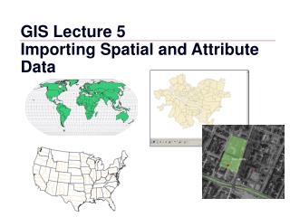
GIS Lecture 5 Importing Spatial and Attribute Data
GIS Lecture 5 Importing Spatial and Attribute Data. Outline. GIS Data Sets Map Projections Coordinate Systems GIS Data Sources. GIS Data Sets. GIS Data Sets. ArcInfo Coverages ArcView Shapefiles CAD Files Aerial Photos Event Files. ArcInfo. AAT Arc Attribute Table

GIS Lecture 5 Importing Spatial and Attribute Data
E N D
Presentation Transcript
GIS Lecture 5 Importing Spatial and Attribute Data
Outline • GIS Data Sets • Map Projections • Coordinate Systems • GIS Data Sources
GIS Data Sets • ArcInfo Coverages • ArcView Shapefiles • CAD Files • Aerial Photos • Event Files
AAT Arc Attribute Table ARC Arc coordinates and topology BND Coverage minimum and maximum coordinates CNT Polygon centroid table PAL Polygon topology PAT Polygon/Point Attribute Table TIC Tic coordinates and Ids DBF Database Table ArcInfo Coverages
Coverage Attribute Table Polygon Coverage
Coverage Attribute Table Point Coverage
Coverage Attribute Table Line Coverages
B E 1 2 Pine St. 733 A 734 F C Oak St. 3 4 D G ArcInfo Coverages • Advantages • Many feature types • Polygons share borders • Area/Perimeter Fields • Disadvantages • Cannot edit in ArcMap
ArcInfo Export files • .e00 export exchange file • ArcCatalog translates into ArcGIS • Creates coverages
ArcView Shape Files • Advantages • heads-up digitizing and editing • less storage/rapid display • can export to CAD • Disadvantages • one feature type • no area or perimeter with new shapefiles
ArcView Shape Files • From 3 to 5 Files • .shp - stores feature geometry • .shx - stores index of features • .dbf - stores attribute data • .sbn and .sbx - store additional indices
CAD Files • Why CAD Drawings? • Better Precision for Digitizing • AutoCAD / Microstation • .DWG / .DXF
Aerial Photos • Combining Grid and Vector Maps
Orthophotography • Digital imagery in which distortion from the camera angle and topography have been removed, thus equalizing the distances represented on the image
GPS • Global Positioning Systems • Earth-orbiting satellites broadcast precisely timed radio signals • GPS receivers determine positions on the ground by calculating distances from three or more satellite transmitters • More expensive than traditional optical and electronic methods
Event Files X,Y Coordinates
Map Projections and Distortion • Map projections produce distortion in one or more spatial properties: • Shape, area, distance, and direction • Specific projections eliminate or minimize distortion
Projection Important • Measurements used to make important decisions • Comparing shapes, areas, distances, or directions of map features • Feature and image themes are aligned New York New York Los Angeles Los Angeles Projection: MercatorDistance: 3,124.67 miles Projection: Albers Equal AreaDistance: 2,455.03 miles Actual distance: 2,451 miles
Projection not Important • Business applications • Not of critical importance. • Concerned with the relative location of different features • On large scale maps - street maps • Distortion may be negligible • Map covers only a small part of the Earth's surface.
Coordinate Systems • Spherical/Polar • Geographic Coordinate System • Rectangular • State Plane • UTM
Geographic Coordinate System • Latitude and Longitude • Census Bureau TIGER files • Geographic • Coordinate • System Grid
Origin • Longitude (prime meridian) 0 • Latitude (equator) 0
Coordinates Pittsburgh 40 -80
Pittsburgh’s Point • Degrees, Minutes, and Seconds (DMS): • 40°26’2”N latitude • -80°0’58”W longitude • Decimal Degrees (DD) • 1 degree = 60 minutes, • 1 minute = 60 seconds • 40°26’2” = • 40 + 26/60 + 2/3600 = 40 + .43333 + .00055 = • 40.434°
Translated to Distance • World circumference through • the poles is 24,859.82 miles, • so for latitude: • 1° = 24,859.82/360 = 69.1 miles • 1’ = 24,859.82/(360*60) = 1.15 miles • 1” = 24,859.82*5,280/(360*3600) = 101 feet • Length of the equator is 24,901.55 miles
Rectangular Coordinate Systems State Plane Coordinates • Local Governments UTM • US Military • Rectangular • Coordinate • System Grid
400 (400, 300) North (Feet) 200 (100, 200) 0 0 200 400 East (Feet) Rectangular Coordinates • Has all positive Cartesian coordinates in feet, called false eastings and false northings
State Plane Coordinate System • Established by the U.S. Coast and Geodetic Survey (now the National Ocean Survey) • At least one for each state • Rectangular (x,y) coordinates • 125 zones, following state and county boundaries each with its own projection: • Lambert conformal projection for zones with east-west extent • Transverse Mercatorprojection for zones with north-south extent • Cannot have zones joined to make larger regions
Universal Transverse Mercator System (UTM) • NIMA - Military grid system • Based on the transverse Mercator projection • Applied to maps of the Earth's surface extending from the Equator to 84 Degrees north and 80 degrees south latitudes
UTM Zones in the Contiguous United States World is divided into 60 north-south zones, each covering a strip 6° wide in longitude
Other Sources of GIS Data • US Census • ESRI Web Sites and Media Kit • Local Agencies • Land Surveys • Satellite Remote Sensing • Existing Paper Maps • Other WEB Sites
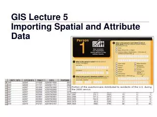
US Census • www.census.gov • TIGER Maps • Summary File(SF) Tables
Census Tracts (TIGER) • Small, relatively permanent statistical subdivisions of counties • delineated by local committees in accordance with Census Bureau guidelines • between 1,000 and 8,000 people (in general) • 1,700 housing units or 4,000 people • homogeneous population characteristics (economic status and living conditions) • normally follow visible features • may follow governmental unit boundaries and other non visible features • more than 60,000 census tracts in Census 2000