Download
1 / 53
530 likes | 573 Vues
Explore proximity buffers for points, lines, polygons, spatial joins with buffers, Visual Basic scripts, apportioning non-coterminous polygons to estimate populations, and advanced calculations for spatial data analysis.

E N D
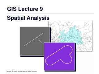
GIS Lecture 9 Spatial Analysis
Outline • Proximity Buffers Points Lines Polygons • Spatial Joins on Buffers • Visual Basic Scripts • Apportioning Non-Coterminous Polygons
Proximity Buffers Created • Points • Lines • Polygons
Points Buffer created by assigning a buffer distance around points
Point Buffer Example - Polygon buffer created ¼ mile around schools
Point Buffer Example • Technology Businesses that are with ¼ mile of Convention Center
Point Buffer Example - Polygon buffer created 20’ around lights - Shows what areas will be lit in a parking lot
Spatial Join - Buffers • Count Faculty and Staff within ¼ mile of University • Spatially join buffers to points • Summarize to count the number of faculty and staff in ¼ mile buffer • Join the buffer count back to the buffer polygon
Lines Buffer created by assigning a buffer distance around lines
Line Buffer Example • Access-to-Work Study (Pittsburgh Foundation) - Polygon buffer created around PAT Bus Routes - Shows 15 minute ride times
Line Buffer Example • Another buffer shows 30 minute ride times
Line Buffer Example …45 minutes
Line Buffer Example …60 minutes
Polygons Buffer created by assigning a buffer distance around polygons
Buffers Buffers Created • Points • Lines • Polygons
Visual Basic Scripts • Adding Area and Perimeter to Polygons • Finding Polygon Centroids
Area and Perimeter VB Script • Advanced calculations for finding area, perimeter, and length of features
Area and Perimeter VB Script • Add field in shapefile (e.g. area) • Use calculator function and Visual Basic Script to calculate polygon areas
Area and Perimeter VB Script • Result is the area of each polygon feature
Polygon Centroids • Advanced calculations for finding polygon centroids • Added as an XY Data Layer
Polygon Centroids • Show the centroids of a polygon • Export attributes as table • Add as XY Data
Polygon Centroids • Create buffers around centroids
Examples of apportionment • You want to know the population of a ZIP code but only have census tracts • Approximate the population of zip codes using Census Tracts or Blocks
Population Apportionment • Begin with census tract population • Overlay zip codes which are non-coterminous • Use apportionment to estimate the population in each census tract • Use census blocks for better estimates
Other examples of apportionment Approximate the population of police zones by using Census Tracts or Blocks
Other examples of apportionment • Approximate the population of voting districts by using Census Tracts or Blocks
Other census data to apportion… • Population (tract and block) • Race (tract and block) • Housing Units (tract and block) • Educational Attainment (tract only) • Income (tract only) • Poverty Status (tract only) • Others?
Tutorial Example: Apportion Data for Non-Coterminous Polygons • Problem: • Police want to know the number of under-educated persons (over Age22) in their car beats • Under-educated data is located in Census tracts (not car beat polygons) • Census tracts and car beats are non-coterminous
Apportion Data for Non-CoterminousPolygons • Apportioning (makes approximate splits) of each tract’s data to two or more car beats.
Approach to Apportionment • Several alternatives for apportioning data -by area (polygons) -length of street network (arcs/lines) -block centroids (points)
Approach to Apportionment • Better to use Census Block data • Areas are smaller than Census Tracts (better population estimates) • Dots are centroids of census blocks • Each dot has censusdata attached to it • Centroids DO NOThave the under-educateddata, census tracts do
Approach to Apportionment Review: • Car beats and census tracts intersect • Census tracts have under-educated data • Census blocks have population data (and are smaller than census tracts, thus better to apportion)
The Math of Apportionment • Zoomed view of 2 car beats and one tract • Beat 261 and 251 • Tract 360550002100
13 block centroids Lie in beat 261 Pop. >22=1,177 13 block centroids Lie in beat 251 Pop. >22=1,089 The Math of Apportionment • Tract 360550002100 • has 205 persons aged 25 or older with less than a HS education • 26 block centroids span 2 beats • Total Population=2,266
The Math of Apportionment • Apportionment assumes that the fraction of under educated persons 25 or older is the same as that for the general population aged 25 or older: • Beat 261: 1,177/2,266 = 0.519 • Beat 251: 1,089/2,266 = 0.481
The Math of Apportionment • 205 is the number of under-educated people in tract 36055002100. • Thus we estimate the contribution of tract 36055002100 to car beat 261’s under-educated population to be (1,177/2,266)x205 = 106. For car beat 251 it is (1,089/2,266)x205 = 99. • To calculate this inGIS, we need to performintersects and joins…
Apportionment Steps • Block Centroids • Add two fields: TRACTID and SumAge22 • TRACTID is a the census tract ID numbers (for later joins and summaries) • SumAge22 is the summary of population Age22+ (calculating multiple age columns)
Apportionment Steps • From the block centroids, create a new summary table counting the number of persons Age22+ for each census tract
Apportionment Steps • Create a new layer intersecting car beats and census tracts • Fields will include values from both tables
Apportionment Steps • Spatially join the new intersecting layer of car beats and census tracts (polygons) to block centroids (points) • New points will have beat and census tract data
Apportionment Steps • Join the summary table of Age22 or greater to the newly created points of car beats, census tracts (block centroid points) • The result is the summary of Age22 or greater population is now on block centroid points