Spatial analysis in GIS
Spatial analysis in GIS. GIS for mineral and hydrocarbon exploration. Used for integrating data (map layers) to identify most prospective areas. ∫. Integrating function linear or non-linear parameters. Output mineral potential map Grey-scale or binary. Input spatial datasets

Spatial analysis in GIS
E N D
Presentation Transcript
GIS for mineral and hydrocarbon exploration Used for integrating data (map layers) to identify most prospective areas ∫ • Integrating function • linear or non-linear • parameters • Output mineral potential map • Grey-scale or binary • Input spatial datasets • Categoric or numeric • Binary or multi-class
Data Types Ratio Interval Ordinal Nominal/categorical Nominal data are items which are differentiated by a simple label, usually a name. May have numbers assigned to them. This may appear ordinal but is not. Nominal items are usually categorical, in that they belong to a definable category. Can be counted, but not ordered or measured. Ordinal data can be ranked (put in order) or have a rating scale attached. Can be counted and ordered, but not measured. Interval data is where the distance between any two adjacent units of measurement (or 'intervals') is the same but the zero point is arbitrary. Ratio data are measured in terms of the ratio between a magnitude of a continuous quantity and a unit magnitude of the same kind. The zero value is absolute
Data Types Parametric vs. Non-parametric Interval and ratio data are parametric, and are used with parametric tools in which distributions are predictable (e.g., Normal). Nominal and ordinal data are non-parametric, and do not assume any particular distribution. They are used with non-parametric tools such as the histogram. 4’ 7” 5’ 5’5” 5’10’ 6’3” 6’8” 4’ 7” 5’ 5’5” 5’10’ 6’3” 6’8” Height of women Height of men Normal distribution – parameters are mean and standard deviation
Data Types Continuous and Discrete Continuous measures are measured along a continuous scale. Discrete data have a set of fixed values. Discreet data Continuous data
Multi-class/continuous and binary data Continuous Binary magnetic map Binary Geological map Multiclass
What is GIS? • GIS = Geographic Information System • Links databases and maps • Manages information about places • Helps answer questions such as: • Where is it? • What else is nearby? • Where is the highest concentration of ‘X’? • Where can I find things with characteristic ‘Y’? • Where is the closest ‘Z’ to my location?
Definition of GIS(Ron Briggs, UT Dallas) A system of integrated computer-basedtoolsfor end-to-endprocessing(capture, storage, retrieval, analysis, display) of data using location on the earth’s surface. • set of integrated tools for spatial analysis • encompasses end-to-end processing of data • capture, storage, retrieval, analysis/modification, display • uses explicit location on earth’s surface to relate data • aimed at decision support, as well as on-going operations and scientific inquiry Because of the link between spatial locations and non-spatial data, it is possible to apply non-spatial statistical modeling methods to spatial data
SPATIAL DATA MODELS What do you mean by spatial data? How real world spatial data are represented? How would you represent a real world river? Land-use?
SPATIAL DATA TYPES • Spatial data comes in three basic forms: • Map data • Attribute data • Image data
SPATIAL DATA TYPES SPATIAL DATA MODELS • Spatial data come in three basic forms: • Map data • Attribute data • Image data Two models: Vector model Raster model
Vector Model: Map data • Map data contains the location and shape of geographic features. Maps use three basic shapes to present real-world features: • points, • lines, and • areas (called polygons/regions).
Vector Model • The spatial locations of features are defined on the basis of coordinate pairs. • These can be discrete, taking the form of points (Point or Node data) or lines (Arc or polylinedata) or areas (Area or polygon data) • Attribute data pertaining the individual spatial features is maintained in an external database. • Topology – A set of rules that models how points, lines and polygons share geometry and are related to each other. Area Population
VECTOR MODEL A Polygon describes a geographic feature that is characterized by a boundary, whether natural, or artificial, such as the boundaries of countries, states, cities, census tracts, postal zones, and market areas or rock types Points represent anything that can be described as an x, y location on earth’s surface, for example, mineral deposits, gas fields Lines objects described by length only (zero width) such as faults, streets, highways, and rivers
SPATIAL DATA TYPES: Image data(Raster Model) Image data ranges from satellite images, digital elevation models, potential field data dataand aerial photographs to scanned maps (maps that have been converted from printed to digital format). We can represent point, line and polygon data in image form
SPATIAL DATA MODELS: Raster Model • Every cell represents a unit area on the ground. All unit areas are equal • The smaller the area the cells represent, the larger the resolution. • Cell values represent a specific property of the ground in that unit area: • For example, • Surface reflectance • Magnetic field • Gravity field • Elevation • Rock type • The values can nominal, ordinal, interval or ratio, they can be integers or floating points. • Georeferenced 10 m x 10 m grid cell
SPATIAL DATA MODELS: Raster Model • Most spatial analysis are done in raster format because it facilitates mathematical calculations, e.g., INGRID1/ INGRID 2 INGRID1 * INGRID 2
VECTOR TO RASTER CONVERSION The area of interest is covered by a fine mesh or matrix of grid cells and the surface attribute value occurring at the centre of each cell point is recorded as the value for that cell. 1 1 3 3 1 2 2 2 3
Raster to vector conversion (Digitization) However, often it is necessary to convert raster to vector format, and then back to the raster format (why??) For vectorization, trace the boundaries using a digitizing tablet/on-screen. Essentially, the X,Y coordinates of features are stored
SPATIAL DATA TYPES: Attribute Data Attribute (tabular) data is the descriptive data that GIS links to map features. Attribute data is collected and compiled for specific areas like states, census tracts, cities, and so on and often comes packaged with map data.
GEOPROCESSING IN GIS • Processing of spatial data to derive predictor map layers • Primary data • Geological map • Structural map • Remote sensing • Geophysical data • geochemical • Derivative (Input) layers • Proximity to granites • Proximity to deep faults • Proximity to fold axes • Reactive rocks • Competency differences • Alteration • Metal anomalies PROCESSING & INTERPRETATION
GEOPROCESSING IN GIS • Querying and conditional evaluation • Density calculations • Distance calculations • Interpolation • Reclassification
QUERYING INGIS • Query by attributes • Query by location
SELECT BY ATTRIBUTES SQL is used for selecting features in a map layer by attributes that full-fill specified condition. for example, SELECT * FROMMapLayerWHERE “field1”>=10 OPTIONS: NEW_SELECTION ADD_TO_SELECTION REMOVE_FROM_SELECTION SUBSET_SELECTION SWITCH_SELECTION IMPORTANT OPERATORS • = • > • < • <> • >= • <= • LIKE • AND • OR • NOT
QUERY BY ATTRIBUTES SELECT * FROM GEOLOGY WHERE “ROCK” =‘Dolerite’ ROCK ROCK
QUERY BY ATTRIBUTES Map of dolerite ROCK
SELECT BY LOCATION Used for selecting features from a map layer based on spatial relationship (adjacency, connectivity, containment) with another layer. For example, SELECT * FROM MapLayer1 CONTAINS MapLayer2 ArcGIS syntax: SelectLayerByLocation MapLayer1 Type_of_relationship MapLayer2 Buffer_distance NEW_SELECTION • Types of spatial relationships that can be queried: • Intersect • Are within a distance of • Contain • Completely contain • Are within • Are completely within • Have their centroid in • Share a line segment with • Are identical to
SELECT BY LOCATION SELECT * FROM GOLD_DEPOSITS WITHIN _ 1_km FROM FAULTS Gold deposits within 1 km from Faults Gold deposits Faults
Density estimation Density is defined as number of (point/line) features per unit area Density surfaces show where point or line features are concentrated. For example, you have a point shape file showing mineral deposit locations. You want to learn more about the metal distribution in the area. Can be used for cluster studies (mineral deposits, population, roads/infrastructure, natural resources such as minerals, forest, agriculture etc., animal inhabitations, ecology…
Density estimation Gold deposits Distribution of gold
Density estimation Faults Faults Fault density (distribution of faults)
Density estimation Distribution of gold Distribution of faults
Distance estimation Euclidean distance is calculated from the center of the source cells to the center of each of the surrounding cells. True Euclidean distance is calculated to each cell in the distance functions. For each cell, the distance is calculated to each source cell by calculating the hypotenuse, with the x-max and y-max as the other two legs of the triangle. This calculation derives the true Euclidean, not cell, distance. The shortest distance to a source is determined, and if it is less than the specified maximum distance, the value is assigned to the cell location on the output raster.
Distance estimation Faults Distance to faults
GEOPROCESSING IN GIS • Interpolation: used for determining the unknown value at any point from the known values at the given sample points in the spatial neigbourhood.
Non-interpolative methods • Interpolative methods
Non-interpolative methods • Assign each sample point to a grid cell (or pixel). • Buffer the sample points. • Draw a Thiessen or Voronoi polygon around each sample point; assign the value at the sample point to the entire area within the Voronoi polygon.
Delaunay triangles a Delaunay triangulation for a set of points is a triangulation of the points in such a way that no point is inside the circumcircle of any triangle. Delaunay triangulations maximize the minimum angle of all the angles of the triangles in the triangulation.
Connecting the centres of the circumcircles produces the Voronoi polygons. The property of a Voronoiploygon of a point is that all points with that polygon are closest to that point. • Voronoi polygons
Interpolation:Estimating values at points intermediate between sample points. • Triangulation • Inverse distance weighting • Natural Neighbours • Krigging
Triangulation • Draw Delaunay triangles for all sample points 5 5 4 4 6 6 3 3 2 2 1 1 The equation for every triangular facet is given by z = a + bx + cy where z is the value, x and y are X and Y coordinates of a sample point, respectively, a, b and c are unknown coefficients Three unknown coefficients, three equations, hence the values of the coefficients can be estimated. Once you have coefficients, you can estimate values at any point within the triangle
Inverse distance weighing 5 4 5 3 6 4 6 2 3 2 1 1 Where z is the value at the point i; w is the weight of i; d(j,i) is the distance between the point iand the point j where the value needs to be calculated; p is the power; n is total number points in the neighbourhood with known values.
Natural neighbor • Natural neighbor interpolation finds the closest subset of sample points for the query point and applies weights to them based on proportionate areas. • Draw Vornoi polygons for all points (green colour) • Draw a Voronoi polygon around the point at which the value is to be determined (orange colour) • Apply weights to each point value in proportion to the area of intersection between the Voronoi polygon of that point and the theVoronoi polygon of the query point. Aijis the area of intersection between the Vornoi polygons of the points i and j.
Krigging The value at the queried point is given by: Where zi are the values at sample points wiare the weights of sample points C● w= D C – Spatial covariance values between the pair of sample points D – Spatial covariances between sample points and the point where the value is required to be estimated C-1● C● w= D ● C-1 Or w= D ● C-1
Krigging: Spatial covariance Covariance between two variables x and y is given by Measures the degree to which x co-varies with y Moment of inertia measures the deviation from the perfect correlation In the above equation, suppose we substitute zt for x and z(t+h) for y, where z is a spatial variable measured at a location t and at another location (t+h), where h is the separation distance called a shift or lag. The spatial covariance of z with itself at separate distance of h can also be measured byγ, (or by C).
Krigging: Variograms By changing the separation distance h (called lag or shift), a series of scatter plots can be generated showing how the variable z is correlated with itself as a function of h. The plot of the moment of inertia as a function of h is called variogram, the plot with covariance is called autocovariance diagram autocovariance diagram Variogram Range Sill Exponential model fitted to the scatter plot Scatter plot γ(h) = C0 if h =0 γ(h) = C0 + C1(1-exp(-3 h/a) ) if h >0 Sill and range are estimated so the model is a reasonable fit to the observed data