Spatial Autocorrelation using GIS
Spatial Autocorrelation using GIS. Jennie Murack murack@mit.edu. Objectives. Understand the concept of spatial autocorrelation Learn which tools to use in Geoda and Arcmap to test for autocorrelation Interpret output from spatial autocorrelation tests.

Spatial Autocorrelation using GIS
E N D
Presentation Transcript
Spatial Autocorrelation using GIS Jennie Murack murack@mit.edu
Objectives • Understand the concept of spatial autocorrelation • Learn which tools to use in Geoda and Arcmap to test for autocorrelation • Interpret output from spatial autocorrelation tests
What is spatial autocorrelation? • Based on Tobler’s first law of geography, “Everything is related to everything else, but near things are more related than distant things.” • It’s the correlation of a variable with itself through space. • Patterns may indicate that data are not independent of one another, violating the assumption of independence for some statistical tests.
Tests for spatial autocorrelation will allow you to answer the following questions about your data: • How are the features distributed? • What is the pattern created by the features? • Where are the clusters? • How do patterns and clusters of different variables compare to one another?
Patterns Useful to: • Better understand geographic phenomena (ex. Habitats) • Monitor conditions (ex. Level of clustering) • Compare different sets of features (ex. Patterns of different types of crimes) • Track change
Patterns You can measure the pattern formed by the location of features or patterns of attribute values associated with features (ex. median home value, percent female, etc.). New AIDS cases in 1994 New AIDS cases in 2003
Types of data often analyzed • Location of crimes, animals, retail, industry, etc. • Land cover • Land use • Census/social data
Software • ArcGIS • Complete GIS software with hundreds of tools • Can work with several datasets (layers) at once. • GeoDa – open source • Solely for spatial statistics • Use one dataset (layer) at a time. • Simple, easy-to-use, interface • Available with registration at: http://geodacenter.asu.edu/
Spatial Neighborhoods and Weights • Neighborhood = area in which the GIS will compare the target values to neighboring values • Neighborhoods are most often defined based on adjacency or distance, but can be defined based on travel time, travel cost, etc. • You can also define a cutoff distance, the amount of adjacency (borders vs. corners), or the amount of influence at different distances • A table of spatial weights is used to incorporate these definitions into statistical analysis.
Distance Models • Inverse distance – all features influence all other features, but the closer something is, the more influence it has • Distance band – features outside a specified distance do not influence the features within the area • Zone of indifference – combines inverse distance and distance band
Adjacency Models • K Nearest Neighbors – a specified number of neighboring features are included in calculations • Polygon Contiguity – polygons that share an edge or node influence each other • Spatial weights – specified by user (ex. Travel times or distances)
Types of Contiguity • Rook = Share edges • Bishop = share corners • Queen = share edges or corners • Secondary order contiguity = neighbor of neighbor Image from: http://www.lpc.uottawa.ca/publications/moransi/moran.htm
Average Nearest Neighbor • Measures how similar the actual mean distance is to the expected mean distance for a random distribution • Measures clustering vs. dispersion of feature locations • Can be used to compare distributions to one another • Concerns: one point on a line is chosen for analysis, extent of study area can affect results (many features near the edge of the study bias results)
Ripley’s K-function • GIS counts the number of neighboring features within a given distance to each feature. • Like Nearest Neighbor, the K-function measures clustering/dispersion of feature locations, but includes neighbors occurring within a certain distance. • It is often used with individual points. • The test compares the observed K value at each distance to the expected K value for a random distribution at each distance. • Concerns: points at the edge of the study area may have few neighbors
Ripley’s K-function Assaults are clustered until about 13,000 ft. and then dispersed beyond 15,000 ft.
Global vs. Local Statistics • Global statistics – identify and measure the pattern of the entire study area • Do not indicate where specific patterns occur • Local Statistics – identify variation across the study area, focusing on individual features and their relationships to nearby features (i.e. specific areas of clustering)
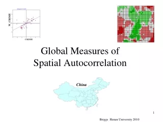
Spatial Autocorrelation (Moran’s I) • Global statistic • Measures whether the pattern of feature values is clustered, dispersed, or random. • Compares the difference between the mean of the target feature and the mean for all features to the difference between the mean for each neighbor and the mean for all features. • For more information on the equation, see ESRI online help Mean of Target Feature Mean of each neighbor Mean of all features
Spatial Autocorrelation (Moran’s I) • Calculates I values: • I=0=random distribution • I<0=Values dispersed • 0<I=Values clustered Clustered Dispersed Random
Spatial Autocorrelation (Moran’s I) I= -.12, slightly dispersed Moran’s I shows the similarity of nearby features through the I value (-1 to 1), but does not indicate if the clustering is for high values or low values. I= .26, clustered
Anselin Local Moran’s I • Local statistic • Measures the strength of patterns for each specific feature. • Compares the value of each feature in a pair to the mean value for all features in the study area. • See ESRI online help for the equation.
Anselin Local Moran’s I • Positive I value: • Feature is surrounded by features with similar values, either high or low. • Feature is part of a cluster. • Statistically significant clusters can consist of high values (HH) or low values (LL) • Negative I value: • Feature is surrounded by features with dissimilar values. • Feature is an outlier. • Statistically significant outliers can be a feature with a high value surrounded by features with low values (HL) or a feature with a low value surrounded by features with high values (LH).
Anselin Local Moran’s I Census tracts for percentage 65 and above Z-scores I values
Getis-Ord General G • Global statistic • Indicates that high or low values are clustered • The value of the target feature itself is not included in the equation so it is useful to see the effect of the target feature on the surrounding area, such as for the dispersion of a disease. • Works best when either high or low values are clustered (but not both). • See ESRI online help for the equation.
Getis-Ord General G High G score: Statistically significant clustering of high values. Low G value: Slight clustering of low values.
Hot Spot Analysis (Getis-OrdGi*) • Local version of the G statistic • The value of the target feature is included in analysis, which shows where hot spots (clusters of high values) or cold spots (clusters of low values) exist in the area. • To be statistically significant, the hot spot or cold spot will have a high/low value and be surrounded by other features with high/low values. • See ESRI online help for the equation.
Hot Spot Analysis (Getis-OrdGi*) Gi* values Z-scores • G=high value=hot spots • G=low value=cold spots
G statistics vs. Local Moran’s I • G statistics are useful when negative spatial autocorrelation (outliers) is negligible. • Local Moran’s I calculates spatial outliers.
G statistics in Geoda • Gi > The value itself at a location (i) is not included in the analysis • Gi* > The value (i) is included in the numerator and denominator.
Permutations in Geoda • Permutation inference is shuffling values around and re-computing statistics each time with a different set of random numbers to construct a reference distribution. • Permutations are used to determine how likely it would be to observe the Moran’s I value of an actual distribution under conditions of spatial randomness. • P-values are dependent on the number of permutations so they are “pseudo p-values”
Reference Distribution • Geoda generates a historgram of the Moran’s I values compared to the observed Moran’s I.
Bivariate Moran’s I • An option in Geoda • It tests 2 variables: the correlation between a given variable (x) at a location and a different variable (y) at surrounding locations. • Results are difficult to interpret. • It is useful in examining the range of interaction provided x and y are correlated at the same location.
Resources • ESRI Spatial Statistics Website: http://blogs.esri.com/Dev/blogs/geoprocessing/archive/2010/07/13/Spatial-Statistics-Resources.aspx • Geoda Workbook: https://geodacenter.asu.edu/system/files/geodaworkbook.pdf • ESRI Spatial Statistics Tool help: http://resources.arcgis.com/en/help/main/10.1/index.html#/An_overview_of_the_Spatial_Statistics_toolbox/005p00000002000000/
ArcMap Help Links • Spatial Autocorrelation (Moran’s I) • http://resources.arcgis.com/en/help/main/10.1/index.html • Anselin Local Moran’s I • http://resources.arcgis.com/en/help/main/10.1/index.html • GetisOrd General G • http://resources.arcgis.com/en/help/main/10.1/index.html • Hot Spot Analysis (GetisOrdGi*) • http://resources.arcgis.com/en/help/main/10.1/index.html