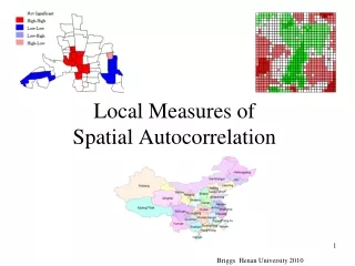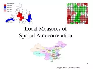
Local Measures of Spatial Autocorrelation
530 likes | 1.76k Vues
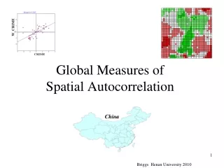
Local Measures of Spatial Autocorrelation. Global Measures and Local Measures. Global Measures (last time) A single value which applies to the entire data set The same pattern or process occurs over the entire geographic area An average for the entire area Local Measures (this time)

Local Measures of Spatial Autocorrelation
E N D
Presentation Transcript
Local Measures ofSpatial Autocorrelation Briggs Henan University 2010
Global Measures and Local Measures • Global Measures (last time) • A single value which applies to the entire data set • The same pattern or process occurs over the entire geographic area • An average for the entire area • Local Measures (this time) • A value calculated for each observation unit • Different patterns or processes may occur in different parts of the region • A unique number for each location China An equivalent local measure can be calculated for most global measures Briggs Henan University 2010
Local Indicators of Spatial Association (LISA) • We will look at local versions of Moran’s I, Geary’s C, and the Getis-Ord G statistic • Moran’s I is most commonly used, and the local version is often called Anselin’s LISA, or just LISA See: Luc Anselin 1995 Local Indicators of Spatial Association-LISAGeographical Analysis 27: 93-115 Briggs Henan University 2010
Local Indicators of Spatial Association (LISA) • The statistic is calculated for each areal unit in the data • For each polygon, the index is calculated based on neighboring polygons with which it shares a border Briggs Henan University 2010
Local Indicators of Spatial Association (LISA) Raw data • Since a measure is available for each polygon, these can be mapped to indicate how spatial autocorrelation varies over the study region • Since each index has an associated test statistic, we can also map which of the polygons has a statistically significant relationship with its neighbors, and show type of relationship LISA Briggs Henan University 2010
Calculating Anselin’s LISA • The local Moran statistic for areal unit i is: where zi is the original variable xi in “standardized form” or it can be in “deviation form” and wij is the spatial weight The summation is across each rowi of the spatial weights matrix. An example follows Briggs Henan University 2010
Example using seven China provinces --caution: “edge effects” will strongly influences the results because we have a very small number of observations Briggs Henan University 2010
Each row in the contiguity matrix describes the neighborhood for that location. 5 4 1 7 6 2 3 Briggs Henan University 2010
Contiguity Matrix and Row Standardized Spatial Weights Matrix 1/3 Briggs Henan University 2010
Calculating standardized (z) scores Briggs Henan University 2010
Calculating LISA wij zj wijzj
Results Moran’s I = -.01889 Raw Data I expected Anhui to be High-Low! (high illiteracy surrounded by low) Low Significance levels are calculated by simulations. They may differ each time software is run. High Low-High
LISA for Illiteracy for all China Provinces Low High Illiteracy Rates LISA Moran’s I = 0.2047 Briggs Henan University 2010
Moran Scatter Plot Scatter Diagram between Xand Lag-X, the “spatial lag” of X formed by averaging all the values of X for the neighboring polygons Identifies which type of spatial autocorrelation exists. Low/High negative SA High/High positive SA Low/Low positive SA High/Low negative SA Briggs Henan University 2010
Quadrants of Moran Scatterplot Each quadrant corresponds to one of the four different types of spatial association (SA) Low/High negative SA High/High positive SA Locations of positive spatial association (“I’m similar to my neighbors”). WX Q2 Q1 Q1 (values [+], nearby values [+]): H-H Q3 (values [-], nearby values [-]): L-L 0 Locations of negative spatial association (“I’m different from my neighbors”). Q3 Q4 X 0 Low/Low positive SA High/Low negative SA Q2 (values [-], nearby values [+]): L-H Q4 (values [+], nearby values [-]): H-L GISC 7361 Spatial Statistics
Why is Moran’s I low for China provinces? • For illiteracy = .2047 • Are provinces really “local” Briggs Henan University 2010
LISA for Median Income, 2000 in D/FW Source: Eric Hajek, 2008 Moran’s I = .59 Briggs Henan University 2010
Examples of LISA for 7 Ohio counties: median income Ashtabula Lake Geauga Cuyahoga Trumbull Summit Portage Ashtabula has a statistically significant Negative spatial autocorrelation ‘cos it is a poor county surrounded by rich ones (Geauga and Lake in particular) Source: Lee and Wong Median Income (p< 0.10) (p< 0.05) Briggs Henan University 2010
Local Getis-Ord G Statistic Local Getis-Ord It is the proportion of all x values in the study area accounted for by the neighbors of location i Global Getis-Ord G Local Moran’s I For comparison G will be high where high values cluster G will be low where low values cluster Interpreted relative to expected value if randomly distributed. Briggs Henan University 2010
LISA and Getis G with Different Distance Weights Data for crime in Columbus, Ohio from Anselin, 1995 LISA with 0,1 contiguity Getis with 1.0 distance Results for Getis G vary depending on distance band used. Getis with 0.5 distance Getis with 2.0 distance
Running in ArcGIS Local Getis G* with Fixed Distance Bands at 2, 1, and 0.5 LISA using Contiguity Weights Briggs Henan University 2010
Can map the statistical significance level and use it as a measure of the “strength” of the spatial autocorrelation --note how the significance level is higher at the center of each cluster. Briggs Henan University 2010
Bivariate LISA Moran Scatter Plot for Crime v. Income • Moran’s I is the correlation between X and Lag-X--the same variable but in nearby areas • Univariate Moran’s I • Bivariate Moran’s I is a correlation between X and a different variable in nearby areas. Moran Significance Map for Crime v. Income Moran Cluster Map for Crime v. Income Briggs Henan University 2010
Scatter Diagram for relationship between income and crime Correlation coefficient r = 0.696 Bivariate LISAand the Correlation Coefficient • Correlation Coefficient is the relationship between two different variables in the same area • Bivariate LISA is a correlation between two different variables in an area and in nearby areas. Bivariate Moran’s I: --less strong relationship --greater scatter --lower slope Moran’s I = -.45 Briggs Henan University 2010
Bivariate LISA: a local version of the correlation coefficient • Can view Bivariate LISA as a “local” version of the correlation coefficient • It shows how the nature & strength of the association between two variables varies over the study region • For example, how home values are associated with crime in surrounding areas Classic Inner City: Low value/ High crime Gentrification? High value/ High crime Unique: Low value/ Low crime Classic suburb: high value/ low crime Briggs Henan University 2010
What have we learned today? Local Indicators of Spatial Autocorrelation • Anselin’s LISA • Local Getis Ord G Spatial autocorrelation can be calculated for each areal unit Spatial autocorrelation can vary across the region in strength and in type Next time (Friday) Using GeoDA software to explore spatial autocorrelation Next week Spatial regression and modeling Briggs Henan University 2010
References • Getis, A. and Ord, J.K. (1992) The analysis of spatial association by use of distance statistics Geographical Analysis, 24(3) 189-206 • Ord, J.K. and Getis A. (1995) Local Spatial Autocorrelation Statistics: distributional issues and an application Geographical Analysis, 27(4) 286-306 • Anselin, L. (1995) Local Indicators of Spatial Association-LISAGeographical Analysis 27: 93-115 Briggs Henan University 2010