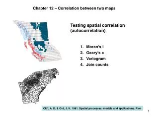
Testing spatial correlation (autocorrelation)
Chapter 12 – Correlation between two maps. Testing spatial correlation (autocorrelation). Moran’s I Geary’s c Variogram Join counts. Cliff, A. D. & Ord, J. K. 1981. Spatial processes: models and applications. Pion. Testing correlation between two maps (continuous variables). x 1. x 2.

Testing spatial correlation (autocorrelation)
E N D
Presentation Transcript
Chapter 12 – Correlation between two maps Testing spatial correlation (autocorrelation) • Moran’s I • Geary’s c • Variogram • Join counts Cliff, A. D. & Ord, J. K.1981. Spatial processes: models and applications. Pion
Testing correlation between two maps (continuous variables) x1 x2 Proportion of land area classified as phydric ln(elevation) in foot Gumpertz, M.L., Wu, C.-T. & Pye J.M. 2000. Logistic regression for southern pine beetle outbreaks with spatial and temporal autocorrelation. Forest Science 95-107.
Assume the correlation coefficient between the two maps is r. The null hypothesis: H0: r = 0. If y = (y1, y2, …, yN) is a random, independent sample, and x = (x1, x2, …, xN)is also an independent sample, the test of H0 is straightforward. Under H0, r has the distribution (N is sample size, e.g., the number of cells): (*) Therefore, p-value for observing an extreme robs is: Equivalently, the test of H0 can be done using a t-test because has a t-distribution. Note these two tests are identical.
However, in reality y = (y1, y2, …, yN) is rarely an independent sample, neither is x = (x1, x2, …, xN). This nuisance is caused by autocorrelation. Autocorrelation inflates type I error. This means two uncorrelated maps will be more likely mistakenly accepted as significantly correlated (reject a true hypothesis). In order to make a correct inference, we need to penalize the sample size. For example, although the sample size is n, the effective sample size should be much smaller than n because of autocorrelation. The effective sample size can be calculated following the method of Clifford et al. (1989), or Dutilleul’s method for small sample size. Clifford, P., Richardson, S. and Hemon, D. 1989. Assessing the significance of the correlation between two spatial processes. Biometrics 45:123-134. Dutilleul, P. 1993. Modifying the t test for assessing the correlation between two spatial processes. Biometric 49:305-314.
covariance distance The effective sample size can be calculated following the method of Clifford et al. (1989). where is a covariance matrix among the n locations. It is a N×N symmetric matrix. It can be estimated by variogram of geostatistics. Calculating the variogram is the most important step to test H0. The major part of computation is to estimate the variogram and the covariance (covariogram) matrix. Covariogram is a decreasing function, i.e., two nearby locations have high covariance than locations far away. Therefore, the covariance matrix captures the spatial correlation structure of the data.
Once we have estimated the covariance matrix, the effective sample size is: Then the test of H0 can follow the same probability distribution as (*), but replace N in (*) by the effective sample size M. The p-value can be as calculated: Note the W-test described in Clifford et al. is very similar to the above test, thus, is not included in my R program. Simply, , and W ~ N(0,1), a standard normal distribution.
Description of R program The main program is called “association.main”. It has five functions. boxcox.fn: boxcoxize the data to make it normality. generatexy.fn: generate a location matrix, and plot the map (image) variogram.fn: calculate empirical variogram for a data varcov.fn: estimate covariance using a theoretical model to fit empirical variogram. test.association.fn: calculate p-value for the test.
Number of recruits Number of species Example: BCI plot – correlation between number of recruits and number of species. Cell size = 10×10 m. Total number of cells N = 5000 Data file name in R: bci.recruit.dat Question of great ecological interest is: Whether diversity (species richness) promotes recruitment and seedling survival? • > bci.recruit.dat[1:10,] • abund nsp recruit simpson • 1 26 22 5 0.9037433 • 2 38 26 12 0.7307692 • 3 57 34 5 0.6086549 • 4 46 29 10 0.5884316 • 5 49 35 12 0.6929293 • 6 52 23 16 0.5067466 • 7 28 24 27 0.8596491 • 8 39 22 10 0.7768131 • 9 57 28 4 0.4071429 • 35 24 2 0.8101852 • … … … … … • 5000 … … … … Wills, C. et al. 2006. Non-random processes contribute to the maintenance of diversity in tropical forests. Science 311:527-531.
Example: BCI plot – correlation between number of recruits and number of species. Cell size = 10×10 m. Total number of cells N = 5000 >association.main(bci.recruit.dat, map1=2, map2=3,cellsize=10,boxcox=“no”) The results are: Correlation coef. r = -0.05455 Original sample size = 5000 p-value = 1e-04 Effective sample size = 1512.2 p-value = 0.0339 map1 = 2 is “number of species”, map2=3 is “number of recruit” The correlation coefficient between the two maps is -0.05455. Without considering autocorrelation, it is highly significant with p-value = 0.0001. After taking account of spatial autocorrelation, it is marginally different from 0, with p-value = 0.0339. (It is significant at p=0.05 level, but not at p=0.001 level.) Note: You need package geoR to run this program.