Intro. To GIS Lecture 6 Spatial Analysis April 8 th , 2013

1. Intro. To GISLecture 6Spatial AnalysisApril 8th, 2013

2. Reminders • Please submit your homework • Project?

3. Spatial Features Types of features in GIS • Point  Nest Site; gas stations • Line  Movement Path; River; • Polygon Home Range; Nest Plot Note: When we talk about features we mean vector datasets

4. Spatial Features cont. • Feature Class • Group of features of the same geometry • Can be filed in different formats Shapefile

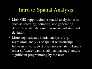
6. Spatial Analysis • The application of operations to coordinate and related attribute data • Maps are great, but this is the real power of GIS • Spatial analysis is used to explore or solve a problem using a variety of geoprocessing tools

7. BASIC SPATIAL ANALYSIS TOOLS IN A GIS • database queries • Selection/selection by location • Spatial joins • basic statistics • Functions (Tools) • Dissolve • Buffering • Near • overlay

8. GIS ANALYSIS TOOLS

9. QUERIES • Ask questions about GIS databases: • Where are the older stands? • Which roads are paved? • Which trails are authorized? • Which water sources are within a certain distance of a road? Note that the queries do not inherently result in a new layer… They usually only highlight features (which could be exported to a new layer afterwards)

10. QUERIES Where are the thinnable stands? Age  30 and Age  40 Age  30 and Age  40 and MBF  30

11. QUERIES • Structured Query Language (SQL) • uses standard operators • e.g. = > < + - * • “and” “or” “not” • standard order of operations • add/subtract before multiply/divide • use parentheses to “isolate” terms

12. QUERIES • Example: • select stands greater than 30 acres with grass understories and a mean quadratic diameter less than 20 inches. • query for above: (area > 30) and (understory = “grass”) and (QMD < 20)

13. QUERIES: Not always the Best Which water sources are within a certain distance of a road? • we need more information. • perhaps a new database layer. • “buffering” may help answer this question

14. Spatial Joins • Joins attributes from one feature class to another based on a spatial relationship(INTERSECT, CONTAINS, WITHIN, CLOSEST) • points in polygon (identifies polygon in which point is located) • polygon in polygon (identifies polygon in which polygon is located) • lines in polygon (identifies polygons crossed by line) • points on lines (calculate distance to nearest line) • points on points (calculate distance to “nearest neighbor” point) • operate on tables and normally creates a new table with additional variables, but does not modify spatial features themselves

15. Query Vs. Spatial Join • Selection: simply selects (“highlights”) entire spatial features in the target layer, but doesn’t modify these features • Selection only • Only Selected features (a subset of all features) are “output” • No new output file saved unless you use Export/data • joins: operate on tables and normally creates a new table with additional fields or variables (columns), but again does not modify actual spatial features (rows) • adds attributes (columns) to the layer’s table from another layer’s table • All features are “output” • No features modified • No new output file saved unless you use Export/data Note: Different approaches can be used, in some cases, to produce same results.

16. BASIC STATISTICS • statistics can help determine meaning within the data • simple, sum, count, mean, maximum, range, variance and standard deviation • calculates statistics for a combination of fields, for example: • by combining the ‘State’ name field & ‘Population’ fields, we can calculate the average state population

17. Right Click on the Field • Go to “Summarize” Choose statistic to summarize

18. BASIC STATISTICS: Calculating Fields • New values can be calculated based on other attribute values • Simple algebra and more advanced math operations • Text functions for picking part of a string or modifying case

19. BASIC STATISTICS: Calculate Geometry • Length, Area, or X,Y coordinates • Choose coordinate system of source or data frame • Pick units of measurement • Make sure field has units in the name

20. Functions (Tools): Types of Analysis

21. Dissolve Tool • Similar to the merge function in Editor toolbar

22. Dissolve Tool • Input Features • Output Feature Class • Dissolve field(s) (optional) • Statistics (optional) • Create multipart features (optional)

23. Buffering • Buffering creates a polygon using a specified distance from a point, line, or other polygon

24. Buffer Tool • Input Features • Output Feature Class • Distance • Linear unit (pick units) • Field (attribute table) • Side/End type • Dissolve Type

25. Buffer application • 500 ft. buffer applied to houses • Buffer overlaps transfer station

26. Multiple-Ring Buffer • Creates buffers for many distances at once • Dissolve option makes them non-overlapping

27. Near Tool • Calculates distance from input features to nearest feature in other layer(s)

28. Near Tool • Output has field with ID and distance of feature • Multiple near layers can be calculated at once • Options to include: • Location (X,Y) • Angle (degrees)

29. Near Application

30. Overlay • Intersect • Identity • Symmetrical Diff. • Union • Clipping/Erasing

31. Intersect (AND Operator) • Polygons split at feature boundaries of both datasets • Only overlapping areas are kept • Attribute tables are updated in output

32. Identity • Similar to intersect but input features are not clipped • Features split along identity polygon edges • Attribute tables are combined in output

33. Symmetrical Difference (XOR Operator) • Simply differencing the two layers (overlapping areas are ignored)

34. Union (OR Operator) • Like Intersect but both input and union features are retained • Output features have attributes from both input and union layers

35. Clipping • Using one layer like a cookie cutter for another • Any vector can be used as input • Clip feature must be a polygon

36. Erasing • The opposite of clipping • Erase feature used to remove a portion of the input data (point, line, or polygon)

37. Intersect / Identity / Union Which function is which?

38. Summary

39. Soil Type Overlaid with Crops Production (ton/ha) Overlay Analysis Overlay Result GIS Technology: Relationship between Land use and Crop Productivity

40. Spatial Analysis Tips • Using these tools in conjunction with each other can produce some useful data • Clip a polygon using a buffer • Calculate new fields to determine percentages • Name your output files so you will remember the inputs and the tool you used • i.e. (LandUse_Buffer_Intersect.shp) • When in doubt, check the help documentation

41. Homework & Lab • HW 7: Ch. 6 p. 149 – 165, answer Q’s 1, 3, 4, 12 • Lab this week: Spatial (vector-raster) Analysis • The instructions will be given (Do NOT bring your lab book on Wed) • Next lecture would be on April 17th