Download
1 / 23
230 likes | 265 Vues
SABER Science, Measurement Approach and Data Product Overview. SABER Science Team. James M. Russell III PI Hampton University Martin G. Mlynczak Associate PI NASA LaRC

E N D
SABER Science, Measurement Approach and Data Product Overview
SABER Science Team James M. Russell III PI Hampton University Martin G. Mlynczak Associate PI NASA LaRC Co-Investigators Ellis E. Remsberg NASA LaRC Doran J. Baker SDL, USU Patrick J. Espy BAS, Cambridge James C. Ulwick SRL, USU Rolando R. Garcia NCAR Raymond G. Roble NCAR David E. Siskind NRL Larry L. Gordley GATS, Inc. Manuel Lopez-Puertas IAA, Spain Richard H. Picard AFRL Christopher J. Mertens NASA LaRC
SABER Science Goal To provide new data and improved understanding of the structure, energetics, chemistry and dynamics of the TIMED core region extending from 60 km to 180 km
SABER Scientific Objectives • Study the M/LT thermal structure and its variations • Implement studies of energetics and radiatively active species in the non-LTE environment • Analyze Oy and HOy chemistry • Conduct dynamics studies
SABER Measurement Objectives • Conduct global-scale, simultaneous, vertical profile measurements of temperature, key chemical constituents, and key emission features, including the following: • - Kinetic Temperature • - O3, H2O, NO, CO2 • - O2(1), OH(u), NO(u), O3(n3), CO2(n2) • - Atomic Species O and H (O inferred 4 different ways) • · Conduct measurements (e.g., T, O3, H2O, CO2) that can be • used to derive and study dynamical quantities such as • geopotential height and potential vorticity • Conduct measurements of O3, H2O, OH(u), O, and H to study ozone and odd hydrogen photochemistry in this region
SABER Measurement Objectives (continued) • Conduct measurements of key radiative emissions to study energetics in the TIMED core region - True cooling: CO2(n2), NO(u), O3(n3), H2O(n2) - Solar heating: O3, O2, CO2(n3) - Chemical heating: O3, O2, OH(u) - Reduction of solar and chemical heating efficiencies: O2(1), OH(u), O3(n3), CO2(n3)
SABER TIMED Science Contributions • Measures T and in the TIMED core region globally • Observes key constituents in the lower portion of the core region globally including O3, H2O, [O], [H] and CO2 • Measures tracer molecules CO2 and H2O for dynamics studies • Measurements made day and night with high vertical resolution (2.2 km IFOV) independently of spacecraft attitude and attitude rate information • Main radiative emission features for energetics are measured: true cooling, chemical heating, solar heating and key emissions that reduce solar and chemical heating efficiency • Observations cover altitude range from the GW source region in the stratosphere, to altitudes where GWs break (~100 km), and in the lower thermosphere
LIMB EMISSION EXPERIMENT VIEWING GEOMETRY AND INVERSION APPROACH Z TANGENT POINT Ho N(Ho) RAY PATH TO SATELLITE }Ho N(Ho) J(x) dx d x d (,q,T,P) dx q known (e.g. CO2) JT J known q (e.g. O3, H2O, CO2…)
# 4 O3 9.3m # 5 H2O6.8m # 6 NO5.3m # 1 CO2- N15.2m # 2 CO2- W15.0m # 3 CO2- W15.0m # 7 CO2 4.26m 1.49o # 8 OH(A) 2.07m # 9 OH(B)1.64m # 10 O2(1) 1.28m 2 km @ 60 km SABER Focal Plane Channel Locations
SABER Daytime Radiance Versus Altitude for 55oS, 287oE, January 8, 2002 300 300 200 200 Tangent Point Altitude (km) 100 100 0 0 -100 -100 Radiance (watts/cm2-sr)
SABER Measurement and Inflight Calibration Cadence • Downscan or upscan every ~53 seconds - ~450 km to ~ –20 km tangent height in ~3.5o latitude • Spacelook Counts updated every ~ 3.5 Minutes • Responsivity updated every ~ 8 Minutes by viewing a hot In-Flight Calibration (IFC) Blackbody
Ground Calibration Scan(BB) 12secs Baffle Scan7secs Gain CycleSpacelook 11secs Adaptive Scan107 secs Space SABER In-flight Calibration System Updates Spacelook Counts Every ~ 3.5 Minutes • Acquisition scan finds the limb • Adaptive scan tracks the limb
Ground IFC to Calibration 7mins 52secs Calibration Scan (BB) Calibration Scan (JS1) Calibration Scan (JS2) Calibration Scan (JS3) Space SABER In-flight Calibration System Updates Responsivity Every ~ 8 Minutes
SABER Views on the Beam of the Spacecraft TIMED spacecraft being prepared for acoustic tests at the NASA Goddard Space Flight Center
Latitude (degrees) Longitude (degrees) SABER Daily Latitude versus Longitude Coverage (83oN - 52oS) North viewing phase of the TIMED yaw cycle
SABER Level 2A Routine Data Products • Vertical profiles of the following parameters day and night: • - Kinetic T, P, density 10 - 105 km - O3 mixing ratio (9.6m) 15 - 100 km • - O3 mixing ratio (1.27m)* 50 - 95 km • - H2O mixing ratio 15 - 80 km • - CO2 (4.3m and 15 m) 85 - 150 km • - NO 5.3m VER** 100 - 180 km • - OH 1.6m VER** 80 - 100 km • - OH 2.0m VER** 80 - 100 km • - O2(1) 1.27m VER** 50 - 105 km • * Day only • ** Volume Emission Rate
- Temperature and Constituent densities • Kinetic T, P, density Z 105 km night and day • [O]concentration • - O3 day / night ‘s 60 - 80 km day • - O2(1) nightglow 80 - 100 km night • - O3(9.6m) / OH(2.0m) 80 - 100 km night • - CO2(4.3m) / CO2(15m) 100 -135 km day • [H] Concentration 80 - 100 km night and day - Cooling Rates • CO2(15m) 20 - 140 km • NO (5.3m) 100 - 180km • O3 (9.6m) 20 - 100 km • H2O (6.7m and far IR) 20 - 70 km SABER Level 2A Analysis Data Products
Solar heating rates, including airglow losses (20 -100 km) • - O3 (Hartley, Huggins, Chappius, and other uv bands) • - O2 (Schumann-Runge, Ly-, Herzberg, and Atmos. Bands) • - CO2 (4.3 m) • Chemical heating rates (80 - 100 km) • - Ox and HOx families • Airglow/Chemiluminescent, Emission/Heating Efficiency • - O2(1) 50 - 105 km • - OH(1.6 m) 80 -100 km • - OH(2.0 m) 80 -100 km • Geostrophic Wind 20 - 100 km SABER Level 2A Analysis Data Products
October 30, 2003 82o N April 20, 2002 82o S Peak energy loss rates are comparable for the two storms Comparison of SABER NO 5.3 mm Energy Loss Rates for April, 2002 and October, 2003 solar storms
SABER Level 3 Data Products • Zonal mean pressure versus latitude cross sections - Orbit, daily, weekly, monthly and seasonally averaged • Polar stereographic and Lambert projection maps on constant pressure and isentropic surfaces - Orbit, daily, weekly, monthly and seasonally averaged maps
SABER NLTE Temperature Zonal Mean Cross Section and global plot on July 9, 2002