Atmospheric phase correction for ALMA
210 likes | 396 Vues
Atmospheric phase correction for ALMA. Alison Stirling John Richer Richard Hills University of Cambridge Mark Holdaway NRAO Tucson. ALMA Goal. To achieve: Diffraction-limited operation at sub-mm wavelengths on baselines up to 14 km. Corresponds to 0.01 arcsec resolution requirement

Atmospheric phase correction for ALMA
E N D
Presentation Transcript
Atmospheric phase correctionfor ALMA Alison Stirling John Richer Richard Hills University of Cambridge Mark Holdaway NRAO Tucson
ALMA Goal To achieve: • Diffraction-limited operation at sub-mm wavelengths on baselines up to 14 km • Corresponds to 0.01 arcsec resolution requirement • To achieve at ALMA’s highest frequencies (~950 GHz), require phase errors < 50 microns on baselines of 14 km • Typical atmospheric phase fluctuations at Chajnantor: 90-400m on 300m baselines at 25-75% level • Corresponds to fluctuations of ~300-1200m at 14km Atmospheric phase correction essential
Atmospheric phase dependence Atmospheric phase fluctuations in sub-mm caused by variations in water vapour and air density
Phase correction strategy To use a combination of: • Fast switching • Measure phase from a nearby point source calibrator • Measures total atmospheric phase • Intermittent (every ~10s of seconds) • Gives phase along a different line of sight • Water vapour radiometry • 183 GHz radiometers four channels • Only sensitive to wet component • Continuous, on source • Two prototype WVRs built by Cambridge and Onsala now ready for testing
Correction Strategy Issues • How often to switch to a calibrator? • Time spent on calibrator? • Angular distance to calibrator? • Smoothing time for WVR brightness temperatures? • Calculation of conversion factor for WVR?
Correction Strategy • Answers depend in detail on atmospheric structure, e.g. • Ratio of wet to dry phase fluctuations • Phase structure function • Also depends on • Instrumental noise (antenna and WVR) • Distribution and brightness of point source calibrators Aim of work: to simulate realistic atmospheric phase fluctuations for the Chajnantor site Day time: 390-1000 m (on 300 m baselines) Night: 90-290m Need separate analysis for day and night time conditions
Met Office Large Eddy Model • Solves Navier-Stokes equation on a grid • Assumes a Kolmogorov energy cascade on sub-grid scales • Models water vapour, temperature, pressure • Two scenarios: • daytime -- convection from surface heating • night time -- wind shear induced turbulence
1.2 . Height / km 0 -2.5 Horizontal distance / km 2.5
2.5 Y / km -2.5 -2.5 X /km 2.5
Location of dry, wet and total refractive index fluctuations Significant anticorrelation between dry and wet Fluctuations at the temperature inversion.
Estimation of fluctuations from radiosonde profiles Solid = total, Dotted wet, Dashed = dry * = Interferometric measurements of total daytime rms phase (Evans et al, 2003) At 50% level: • Dry: 200 microns • Wet: 400 microns • Total: 400 microns • Independent confirmation of phase fluctuation amplitude • Initial estimates of dry fluctuation component
Daytime structure function • Solid = dry • Dot dashed = wet • Dotted = cross-correlation term • Consistent with Kolmogorov spectrum on small scales
Nocturnal mean profiles Gradient of temperature profile opposite sign from water vapour profile
Evolution of night time fluctuations 0.6 Height / km 0 Horizontal distance / km -0.3 0.3
Location of dry, wet and total refractive index fluctuations Negative correlation between wet and dry fluctuations near ground
Nocturnal structure function • Blue dashed = wet; black solid = dry • r.m.s. wet fluctuations ~ 2 x r.m.s dry • Exponent of wet: 1.0, dry: 0.8 • Turn over around 800m (~ depth of layer)
Simulations of phase correction • AIPS++ code written by Mark Holdaway • Combines Mark’s fast switching simulator with our 3-D simulations of atmosphere • WVR simulated using `am’ radiative transfer code to calculate brightness temperatures (Scott Paine)
Conclusions • Now have realisations of the atmosphere at Chajnantor for day and night conditions • Dry and wet fluctuations have different distributions depending on time of day • Have developed simulations of FS+WVR phase correction • Future plans: • Investigate different phase correction strategies • Validation of the two ALMA prototype WVRs on SMA