Kernels, Margins, and Low-dimensional Mappings
160 likes | 300 Vues
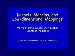
Kernels, Margins, and Low-dimensional Mappings. Maria-Florina Balcan, Avrim Blum, Santosh Vempala. [NIPS 2007 Workshop on TOPOLOGY LEARNING ]. Generic problem. Given a set of images: , want to learn a linear separator to distinguish men from women.

Kernels, Margins, and Low-dimensional Mappings
E N D
Presentation Transcript
Kernels, Margins, and Low-dimensional Mappings Maria-Florina Balcan, Avrim Blum, Santosh Vempala [NIPS 2007 Workshop on TOPOLOGY LEARNING ]
Generic problem • Given a set of images: , want to learn a linear separator to distinguish men from women. • Problem: pixel representation no good. Old style advice: • Pick a better set of features! • But seems ad-hoc. Not scientific. New style advice: • Use a Kernel! K( , ) = ()¢( ). is implicit, high-dimensional mapping. • Feels more scientific. Many algorithms can be “kernelized”. Use “magic” of implicit high-dim’l space. Don’t pay for it if exists a large margin separator.
Generic problem Old style advice: • Pick a better set of features! • But seems ad-hoc. Not scientific. New style advice: • Use a Kernel! K( , ) = ()¢ (). is implicit, high-dimensional mapping. • Feels more scientific. Many algorithms can be “kernelized”. Use “magic” of implicit high-dim’l space. Don’t pay for it if exists a large margin separator. • E.g., K(x,y) = (x ¢ y + 1)m. :(n-diml space) ! (nm-diml space).
Claim: Can view new method as way of conducting old method. • Given a kernel [as a black-box program K(x,y)] and access to typical inputs [samples from D], • Claim: Can run K and reverse-engineer an explicit (small) set of features, such that if K is good [9 large-margin separator in -space for D,c], then this is a good feature set[9 almost-as-good separator]. “You give me a kernel, I give you a set of features” Do this using idea of random projection…
Claim: Can view new method as way of conducting old method. • Given a kernel [as a black-box program K(x,y)] and access to typical inputs [samples from D], • Claim: Can run K and reverse-engineer an explicit (small) set of features, such that if K is good [9 large-margin separator in -space for D,c], then this is a good feature set[9 almost-as-good separator]. E.g., sample z1,...,zd from D. Given x, define xi = K(x,zi). Implications: • Practical: alternative to kernelizing the algorithm. • Conceptual: View kernel as (principled) way of doing feature generation. View as similarity function, rather than “magic power of implicit high dimensional space”.
Basic setup, definitions + - + - w X • Instance space X. • Distribution D, target c. Use P = (D,c). • K(x,y) = (x)¢(y). • P is separable with margin g in -space if 9 w s.t. Pr(x,l)2 P[l(w¢(x)/|(x)|) <g]=0. (|w|=1) • Error e at margin g: replace “0” with “e”. Goal is to use K to get mapping to low-dim’l space. P=(D,c)
One idea: Johnson-Lindenstrauss lemma + - + - + - + - X P=(D,c) • If P separable with margin g in f-space, then with prob 1-d, a random linear projection down to space of dimension d = O((1/g2)log[1/(de)]) will have a linear separator of error < e. [Arriaga Vempala] • If vectors are r1,r2,...,rd, then can view as features xi = (x)¢ ri. • Problem: uses . Can we do directly, using K as black-box, without computing ?
3 methods (from simplest to best) • Draw d examples z1,...,zd from D. Use: F(x) = (K(x,z1), ..., K(x,zd)). [So, “xi” = K(x,zi)] For d = (8/e)[1/g2 + ln 1/d], if P was separable with margin g in -space, then whp this will be separable with error e. (but this method doesn’t preserve margin). • Same d, but a little more complicated. Separable with error e at margin g/2. • Combine (2) with further projection as in JL lemma. Get d with log dependence on 1/e, rather than linear. So, can set e¿ 1/d. All these methods need access to D, unlike JL. Can this be removed? We show NO for generic K, but may be possible for natural K.
Key fact Claim:If 9 perfect w of margin g in f-space, then if draw z1,...,zd2 D for d ¸ (8/e)[1/g2 + ln 1/d], whp (1-d) exists w’ in span((z1),...,(zd)) of error ·e at margin g/2. Proof:Let S = examples drawn so far. Assume |w|=1, |(z)|=18 z. • win = proj(w,span(S)), wout = w – win. • Say wout is large if Prz(|wout¢(z)| ¸g/2)¸e; else small. • If small, then done: w’ = win. • Else, next z has at least e prob of improving S. |wout|2Ã |wout|2 – (g/2)2 • Can happen at most 4/g2 times. □
So.... If draw z1,...,zd2 D for d = (8/e)[1/g2 + ln 1/d], then whp exists w’ in span((z1),...,(zd)) of error ·e at margin g/2. • So, for some w’ = a1(z1) + ... + ad(zd), Pr(x,l) 2 P [sign(w’ ¢(x)) ¹l] ·e. • But notice that w’¢(x) = a1K(x,z1) + ... + adK(x,zd). ) vector (a1,...ad) is an e-good separator in the feature space: xi = K(x,zi). • But margin not preserved because length of target, examples not preserved.
How to preserve margin? (mapping #2) • We know 9w’ in span((z1),...,(zd)) of error ·e at margin g/2. • So, given a new x, just want to do an orthogonal projection of (x) into that span. (preserves dot-product, decreases |(x)|, so only increases margin). • Run K(zi,zj) for all i,j=1,...,d. Get matrix M. • Decompose M = UTU. • (Mapping #2) = (mapping #1)U-1. □
Mapping #2, Details • Draw a set S={z1, ..., zd} of d = (8/e)[1/g2 + ln 1/d], unlabeled examples from D. • Run K(x,y) for all x,y2S, get M(S)=(K(zi,zj))zi,zj2 S. • Place S into d-dim. space based on K (or M(S)). Rd F2(z3) X K(z1,z1)=|F2(z1)|2 K(z3,z3) z3 z1 F2(z1) F1 K(z1,z2) z2 F2(z2) K(z2,z2)
Mapping #2, Details, cont • What to do with new points? • Extend the embedding F1to all of X: • consider F2: X ! Rd defined as follows: for x 2 X, let F2(x) 2 Rd be the point of smallest length such that F2(x) ¢F2(zi) = K(x,zi), for all i 2 {1, ..., d}. • The mapping is equivalent to orthogonally projecting (x) down to span((z1),…, (zd)).
How to improve dimension? • Current mapping (F2) gives d = (8/e)[1/g2 + ln 1/d]. • Johnson-Lindenstrauss gives d1 = O((1/g2) log 1/(de) ). Nice because can have d¿ 1/. • Answer: just combine the two... • Run Mapping #2, then do random projection down from that. • Gives us desired dimension (# features), though sample-complexity remains as in mapping #2.
RN X X O O O X X X O Rd X O F2 X O X X O X O X X JL X X X X O O O F O Rd1 X O X O X X O X O
Open Problems • For specific natural kernels, like K(x,y) = (1 + x¢y)m, is there an efficient analog to JL, without needing access to D? • Or, at least can one at least reduce the sample-complexity ? (use fewer accesses to D) • Can one extend results (e.g., mapping #1: x [K(x,z1), ..., K(x,zd)]) to more general similarity functions K? • Not exactly clear what theorem statement would look like.