The Dvorak Technique
The Dvorak Technique. The Dvorak Technique. Originally By: TSgt Johnson (JTWC Satellite Operations) Updated by Mr. Paul McCrone (HQ AFWA/XOGM). The Dvorak Technique. Positioning Intensity Estimation Final T-number Data-T Pattern-T Model-T Current Intensity Coding. Eye


The Dvorak Technique
E N D
Presentation Transcript
The Dvorak Technique The Dvorak Technique Originally By: TSgt Johnson (JTWC Satellite Operations) Updated by Mr. Paul McCrone (HQ AFWA/XOGM)
The Dvorak Technique • Positioning • Intensity Estimation • Final T-number • Data-T • Pattern-T • Model-T • Current Intensity • Coding
Eye Exposed Low Level Circulation Center (LLCC) Central Dense Overcast (CDO) Embedded Center (EMB CTR) Spiral Band Curvature (SBC) Partially exposed LLCC Cloud minimum wedge Central Cold Cover (CCC) Cirrus outflow Circle method Conservative feature Animation Extrapolation Positioning
Low Level Circulation CenterLLCC Low Level Cloud LinesLLCLS Upper Level Circulation CenterULCC Central Dense OvercastCDO Embedded CenterEMB CTR Spiral Band CurvatureSBC Central Cold CoverCCC Enhanced Infrared EIR Convection CNVCTN Common Abbreviations
Dark cloud free spot Shadowy spot for cloud filled eye Without LLCC showing within eye, fix on center of eye Measure width Evaluate shape Eye Fixes Visual (VIS)
IR Warm spot As a guideline look for 2 shades warmer on the BD curve (MUST use BD CURVE!) Use warmest spot. Eye boundary (eye wall)defined by the tightest temperature gradient Measure width and shape independent of Visual. Eye Fixes Infrared (IR)
Look for tightening cyclonic low clouds. The center will be within the tightest circle of clouds. Much easier to find with VIS imagery Exposed LLCC Fixes
VIS only (The term “CDO” implies “VIS only” - no exceptions! Look for low level cloud lines to extrapolate underneath convection Look for overshooting tops - bias LLCC toward tallest tops! Look for SBC pattern in texture of CDO CDO Fixes
Look for a warm spot Look toward the edge with the tightest temperature gradient Don’t forget continuity with past positions EMB CTR
Draw Streamlines on the image. Place each streamline so the curve lies as close as possible to the low level cloud lines (LLCLS) and convective bands. Follow the streamlines to the center. SBC Fixes VIS
Draw Streamlines on the image. Place each streamline so the curve lies as close as possible to the low level cloud lines (LLCLS) and convective bands. Follow the streamlines to the center. SBC Fixes VIS
Draw Streamlines on the image. Place each streamline so the curve lies as close as possible to the low level cloud lines (LLCLS) and connective bands. Follow the curves to the center Same idea as VIS SBC Fixes IR
Defined as “Less than half of the LLCC exposed” Includes cirrus obscuration The center will be within the tightest circle of clouds. Similar to the Fully exposed LLCC, just harder - less obvious. Partially Exposed LLCC Fixes VIS
Again…. “Less than half of the LLCC exposed” Same idea as visual, except this can be even harder LLCLS don’t show up well in GOES/GMS EIR (but they show up fairly well in DMSP Thermal imagery). Partially Exposed LLCC Fixes IR
The center will be halfway along a line drawn from the tip of the wedge straight across the comma head. Cloud Minimum Wedge
The center will be halfway along a line drawn from the tip of the wedge straight across the comma head. Cloud Minimum Wedge Dry Slot
The center will be halfway along a line drawn from the tip of the wedge straight across the comma head. Cloud Minimum Wedge
The center will be halfway along a line drawn from the tip of the wedge straight across the comma head. Cloud Minimum Wedge
The center will be halfway along a line drawn from the tip of the wedge straight across the comma head. Cloud Minimum Wedge
The center will be halfway along a line drawn from the tip of the wedge straight across the comma head. Cloud Minimum Wedge
Rare; to be used with VIS imagery ONLY Typically, storm exhibits a milky cirrus top - few convective cells visible Only use if there is no evidence of the CDO or curved lines visible through the cirrus. Center placement based mostly on continuity. CCC Fixes VIS
Very difficult to accurately locate center. Center placement based mostly on continuity. CCC Fixes IR
Use only when low clouds are not visible. Follow the cirrus outflow anticyclonically back to the center. This locates the Upper Level Circulation Center (ULCC) ONLY USE AS A LAST RESORT. Cirrus Outflow Fixes
To be used with weak or very broad systems. Use all available curvature to find center. Where most circles meet, indicates most likely LLCC. Circle Method Fixes
If you had good reason to believe the LLCC was located at a certain point in relationship with a persistent feature, the LLCC will remain in the same relative location for up to 12 hours (at the very furthest in time) Conservative Features Fixes
Self explanatory Use with all type of fixes when available. Use animation alone only when still imagery gives no indication of LLCC. Animation Fixes
Extrapolate past few fixes to determine where current position should be located. Limited by the accuracy of the past fixes Don’t technically need a satellite image to do this This is a mathematical “dead-reckoning” approach. This method is not encouraged as an analysis method Extrapolation Fixes
Step 1 - Locate Cloud System Center (CSC) Step 2 - Determine the Data Type (Data-T) Step 3 - CCC Step 4 - Past 24 hour trend Step 5 - Model Expected T-number (MET) Step 6 - Pattern T-number (PT) Step 7 - T-number determination Step 8 - Final-T Step 9 - Current Intensity (CI) Step 10 - Final-T/CI encoding Intensity Estimation
Step 2A Curved Band Step 2B Shear Pattern Step 2C Eye Pattern Step 2D CDO Step 2E Embedded Center Step 2, Data-T
Use a LOG10 spiral overlay. The spiral should lie along the axis of the of the band, and roughly parallel the inside edge of the band. Measure the arc length. Step 2A, Curved Band
Use a LOG10 spiral overlay. The spiral should lie along the axis of the of the band, and roughly parallel the inside edge of the band. Measure the arc length. Step 2A, Curved Band
Measuring the arc length: Follow the convection, not cirrus blow-off Easier to do with Visual than Enhanced IR. You may have small breaks in convection and draw through Step 2A, Curved Band
Use a LOG10 spiral overlay. The spiral should lie along the axis of the of the band, and roughly parallel the inside edge of the band. Measure the arc length. Step 2A, Curved Band LOG10 Spiral
Measuring the arc length: Can be very subjective Inexperienced analysts tend to go too high (fooled by cirrus). This storm is somewhere between 0.70 and 0.85. Step 2A, Curved Band
Step 2A, Curved Band Note: Southern Hemisphere Example
Step 2A, Curved Band Note: Southern Hemisphere Example
Step 2A, Curved Band Note: Southern Hemisphere Example
Step 2A, Curved Band Draw your banding line from the outside , then in.
Step 2A, Curved Band 0.70 0.80 0.60 0.50 Start from your LLCC and count “pie slices” or log10 sectors. They are counted in tenths. 360 degrees around equals “1.00” wrap 0.40 0.10 0.30 0.20
A wrap of 0.80 would equal a Data T of T3.5 Step 2A, Curved Band 0.70 0.80 0.60 0.50 0.40 0.10 0.30 0.20
I could have added an additional 0.05 for this portion of wrap, giving a total wrap of 0.85 - Judgement call. 0.70 0.80 0.60 0.50 0.40 0.10 0.30 0.20
Measure the distance from the LLCC to the nearest convection. In IR, use the dark gray(DG) shade on BD Curve ONLY to identify convection. Step 2B, Shear Pattern
Measure the distance from the LLCC to the nearest convection. In EIR, use the dark gray(DG) on BD Curve ONLY shade to identify convection. Step 2B, Shear Pattern 70nm = T1.5
Terms E#: Eye Number Eye adj: Eye adjustment CF: Central Feature BF: Banding Feature CF Formula: CF = E# + Eye adj Data-T Formula: DT = CF + BF Step 2C, Eye Pattern
Step 2C (E# VIS) • Determine if Eye is banding type or not. • Measure the embedded distance of the eye, or the average band width if eye is a banding type. • For small eyes, measure distance from center. • For large eyes (> 30 nm) measure from edge. • Apply Values to E# Table
CDO type eye CDO
CDO type eye CDO Measure narrowest distance (This is for a Large eye, which defined as 30 nm or more inclusive)
CDO type eye CDO Measure narrowest distance (This is for a SMALL eye, which defined as 29 nm or less)