Scalable Analytic Models for Cloud Services

1. Scalable Analytic Models for Cloud Services RahulGhosh PhD student, Duke University , USA Research intern, IBM T. J. Watson Research Center, USA E-mail: rahul.ghosh@duke.edu NEC Research Lab, Tokyo, Japan December 15, 2010

2. Acknowledgments • Collaborators • Prof. Kishor S. Trivedi (advisor) • Dr. Vijay K. Naik (mentor at IBM Research) • Dr. DongSeong Kim (post-doc in research group) • Francesco Longo (visiting PhD student in research group) • This research is financially supported by NSF and IBM Research

3. Talk outline • An Overview of Cloud Computing • Different definitions and key characteristics • Evolution of cloud computing • Motivation • Key challenges and goals of our work • Performability Analysis of IaaS Cloud • Joint analysis of performance and availability using interacting stochastic models • Future Research • Conclusions

4. Talk outline • An Overview of Cloud Computing • Different definitions and key characteristics • Evolution of cloud computing • Motivation • Key challenges and goals of our work • Performability Analysis of IaaS Cloud • Joint analysis of performance and availability using interacting stochastic models • Future Research • Conclusions

5. NIST definition of cloud computing • Cloud computing is a model of Internet-based computing • Definition provided by National Institute of Standards and Technology (NIST): • “Cloud computing is a model for enabling convenient, • on-demand network access to a shared pool of configurable computing resources (e.g., networks, servers, storage, applications, and services) that can be rapidly provisioned and released with minimal management effort or service provider interaction.” • Source: P. Mell and T. Grance, “The NIST Definition of Cloud Computing”, October 7, 2009

6. NIST definition of cloud computing • Cloud computing is a model of Internet-based computing • Definition provided by National Institute of Standards and Technology (NIST): • “Cloud computing is a model for enabling convenient, • on-demand network access to a shared pool of configurable computing resources (e.g., networks, servers, storage, applications, and services) that can be rapidly provisioned and released with minimal management effort or service provider interaction.” • Source: P. Mell and T. Grance, “The NIST Definition of Cloud Computing”, October 7, 2009

7. Key characteristics • On-demand self-service: • Provisioning of computing capabilities, without human interactions • Resource pooling: • Shared physical and virtualized environment • Rapid elasticity: • Through standardization and automation, quick scaling at any time • Metered Service: • Pay-as-you-go model of computing • Source: P. Mell and T. Grance, “The NIST Definition of Cloud Computing”, October 7, 2009 Many of these characteristics are borrowed from Cloud’s predecessors!

8. Evolution of cloud computing • Cloud is NOT a brand new concept • Rather it is a technology whose “tipping point” has come* • Time line of evolution Around 2005-06 Around 2000 Cloud computing Early 90s Utility computing Early 60s Grid computing Cluster computing What are the key characteristics of these early models which are inherited by Cloud? • *Source: http://seekingalpha.com/article/167764-tipping-point-gartner-annoints-cloud-computing-top-strategic-technology

9. Grid vs. cloud computing • Both are highly distributed computing resources and need to manage very large facilities . • Key components which distinguish a cloud from a grid are: virtualization and standardization /automation of resource provisioning steps. • Cloud service providers can reduce their costs of service delivery by resource consolidation (through virtualization) and by efficient management strategies (through standardization and automation). • Users of cloud service can also reduce the cost of computing due to a pay-as-you-go pricing model, where the users are charged based on their computing • demand and duration of resource holding.

10. Cloud Service models • Infrastructure-as-a-Service (IaaS) Cloud: • Examples: Amazon EC2, IBM Smart Business Development and Test Cloud • Platform-as-a-Service (PaaS) Cloud: • Examples: Micorsoft Windows Azure, Google AppEngine • Software-as-a-Service (SaaS) Cloud: • Examples: Gmail, Google Docs

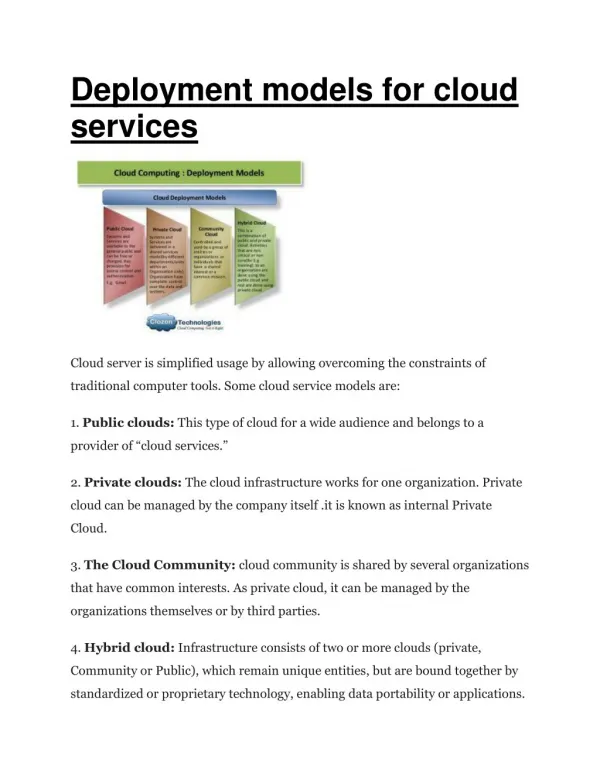
11. Deployment models • Private Cloud: • Cloud infrastructure solely for an organization • Managed by the organization or third party • May exist on premise or off-premise • Public Cloud: • Cloud infrastructure available for use for general users • Owned by an organization providing cloud services • Hybrid Cloud: • - Composition of two or more clouds (private or public)

12. Talk outline • An Overview of Cloud Computing • Different definitions and keycharacteristics • Evolution of cloud computing • Service and deployment models, enabling technologies • A quick look into Amazon’s cloud service offerings • Motivation • Key challenges and goals of our work • Performability Analysis of IaaS Cloud • Joint analysis of performance and availability using interacting stochastic models • Future Research • Conclusions

13. Key challenges • Two critical obstacles of a cloud: • Service (un)availability and performance unpredictability • Large number of parameters can affect performance and availability • Nature of workload (e.g., arrival rates, service rates) • Failure characteristics (e.g., failure rates, repair rates, modes of recovery) • Types of physical infrastructure (e.g., number of servers, number of cores per server, RAM and local storage per server, configuration of servers, network configurations) • Characteristics of virtualization infrastructures (VM placement, VM resource allocation and deployment) • Characteristics of different management and automation tools Performance and availability assessments are difficult!

14. Common approaches • Measurement-based evaluation: • Appealing because of high accuracy • Expensive to investigate all variations and configurations • Time consuming to observe enough events (e.g., failure events) to get statistically significant results • Lacks repeatability because of sheer scale of cloud • Discrete-event simulation models: • Provides reasonable fidelity but expensive to investigate many alternatives with statistically accurate results • Analytic models: • -Lower relative cost of solving the models • -May become intractable for a complex real sized cloud • -Simplifying the model results in loss of fidelity

15. Our goals • Developing a comprehensive modeling approach for joint analysis of availability and performance of cloud services • Developed models should have high fidelity to capture all the variations and configuration details • Proposed models need to be tractable and scalable • Applying these models to solve cloud design and operation related problems

16. Talk outline • An Overview of Cloud Computing • Different definitions and keycharacteristics • Evolution of cloud computing • Service and deployment models, enabling technologies • A quick look into Amazon’s cloud service offerings • Motivation • Key challenges and goals of our work • Performability Analysis of IaaS Cloud • Joint analysis of performance and availability using interacting stochastic models • Future Research • Conclusions

17. Key problems of interest: Characterize cloud services as a function of arrival rate, available capacity, service requirements, and failure properties Apply these characteristics in cloud capacity planning, SLA analysis and management, energy-response time tradeoff analysis, cloud economics Proposed approach: Designing analytical models that allow us to capture all the important details of the workload, fault load and system hardware/software/manage aspects to gain fidelity and yet retain tractability Two service quality measures: service availability and provisioning response delay These service quality measures are performability measures in a sense that they take into account contention for resources as well as failure of resources Introduction

18. Motivation behind this approach: Measurement based evaluation of the QoS metrics is difficult, because: it requires extensive experimentation with each workload, system configuration it may not capture enough failure events to quantify the effects of resource failures Analytic modeling of cloud service is considered to be difficult due to largeness and complexity of service architecture We use interacting Markov chain based approach Lower relative cost of solving the models while covering large parameter space Our approach is tractable and scalable Introduction We describe a general approach to performability analysis applicable to variety of IaaS clouds using interacting stochastic process models

19. Novelty of our approach • Single monolithic model vs. interacting sub-models approach • Even with a simple case of 6 physical machines and 1 virtual machine per physical machine, a monolithic model will have 126720 states. • In contrast, our approach of interacting sub-models has only 41 states. Clearly, for a real cloud, a naïve modeling approach will lead to very large analytical model. Solution of such model is practically impossible. Interacting sub-models approach is scalable, tractable and of high fidelity. Also, adding a new feature in an interacting sub-models approach, does not require reconstruction of the entire model. What are the different sub-models? How do they interact?

20. Main Assumptions All requests are homogenous, where each request is for one virtual machine (VM) with fixed size CPU cores, RAM, disk capacity. We use the term “job” to denote a user request for provisioning a VM. Submitted requests are served in FCFS basis by resource provisioning decision engine (RPDE). If a request can be accepted, it goes to a specific physical machine (PM) for VM provisioning. After getting the VM, the request runs in the cloud and releases the VM when it finishes. To reduce cost of operations, PMs can be grouped into multiple pools. We assume three pools – hot (running with VM instantiated), warm (turned on but VM not instantiated) and cold (turned off). All physical machines (PMs) in a particular type of pool are identical. System model

21. Provisioning and servicing steps: (i) resource provisioning decision, (ii) VM provisioning and (iii) run-time execution Life-cycle of a job inside a IaaS cloud Provisioning response delay VM deployment Provisioning Decision Actual Service Out Arrival Queuing Instantiation Resource Provisioning Decision Engine Run-time Execution Instance Creation Deploy Job rejection due to buffer full Job rejection due to insufficient capacity We translate these steps into analytical sub-models

22. Resource provisioning decision Provisioning response delay Resource Provisioning Decision Engine VM deployment Provisioning Decision Actual Service Out Run-time Execution Arrival Queuing Instantiation Instance Creation Deploy Admission control Job rejection due to buffer full Job rejection due to insufficient capacity

23. Flow-chart: Resource provisioning decision engine (RPDE)

24. Resource provisioning decision model: CTMC 0,h 1,h N-1,h i,s i = number of jobs in queue, s = pool (hot, warm or cold) … 0,0 0,w 1,w N-1,w … N-1,c 0,c 1,c …

25. Resource provisioning decision model: parameters & measures • Input Parameters: • –arrival rate: data collected from publicly available cloud • – mean search delays for resource provisioning decision engine: from searching algorithms or measurements • – probability of being able to provision: computed from VM provisioning model • N – maximum # jobs in RPDE: from system/server specification • Output Measures: • Job rejection probability due to buffer full (Pblock) • Job rejection probability due to insufficient capacity (Pdrop) • Total job rejection probability (Preject= Pblock+ Pdrop) • Mean queuing delay for an accepted job (E[Tq_dec]) • Mean decision delay for an accepted job (E[Tdecision])

26. VM provisioning Provisioning response delay Resource Provisioning Decision Engine VM deployment Provisioning Decision Actual Service Out Run-time Execution Arrival Queuing Instantiation Instance Creation Deploy Admission control Job rejection due to buffer full Job rejection due to insufficient capacity

27. VM provisioning model Hot PM Hot pool Resource Provisioning Decision Engine Warm pool Service out Accepted jobs Running VMs Idle resources in hot machine Cold pool Idle resources in warm machine Idle resources in cold machine

28. VM provisioning model for each hot PM Lh is the buffer size and m is max. # VMs that can run simultaneously on a PM 0,0,0 0,1,0 Lh,1,0 … 0,0,1 (Lh-1),1,1 Lh,1,1 … … … … … … … … 0,0,(m-1) 0,1,(m-1) (Lh-1),1,(m-1) Lh,1,(m-1) … 0,0,m 1,0,m Lh,0,m i = number of jobs in the queue, j = number of VMs being provisioned, k = number of VMs running i,j,k

29. VM provisioning model (for each hot PM) • Input Parameters: • can be measured experimentally • obtained from the lower level run-time model • obtained from the resource provisioning decision model • Hot pool model is the set of independent hot PM models • Output Measure: • = prob. that a job can be accepted in the hot pool = • where, is the steady state probability that a PM can accept job for provisioning - from the solution of the Markov model of a hot PM on the previous slide

30. VM provisioning model for each warm PM 0,0,0 0,1*,0 Lw,1*,0 … 0,1,0 Lw,1,0 … 0,1**,0 Lw, 1**,0 … … … … … 0,1,1 … … 0,0,1 (Lw-1),1,1 Lw,1,1 … 0,0,(m-1) 0,1,(m-1) (Lw-1),1,(m-1) Lw,1,(m-1) … 0,0,m 1,0,m Lw,0,m

31. VM provisioning model for each cold PM 0,0,0 0,1*,0 Lc,1*,0 … 0,1,0 Lc,1,0 … 0,1**,0 Lc, 1**,0 … … … … … 0,1,1 … 0,0,1 (Lc-1),1,1 Lc,1,1 … … 0,0,(m-1) 0,1,(m-1) (Lc-1),1,(m-1) Lc,1,(m-1) … 0,0,m 1,0,m Lc,0,m

32. VM provisioning model: Summary • For warm/cold PM, the VM provisioning model is similar to hot PM, with the following exceptions: • Effective job arrival rate • For the first job, warm/cold PM requires additional start-up work • Mean provisioning delay for a VM for the first job is longer • Buffer sizes are different • Outputs of hot, warm and cold pool models are the steady state probabilities that at least one PM in hot/warm/cold pool can accept a job for provisioning. These probabilities are denoted by and respectively • From VM provisioning model, we can also compute mean queuing delay for VM provisioning (E[Tvm_q]) and conditional mean provisioning delay (E[Tprov]). • Net mean response delay is given by: (E[Tresp]=E[Tq_dec]+E[Tdecision]+E[Tq_vm]+E[Tprov])

33. Run-time execution Provisioning response delay Resource Provisioning Decision Engine VM deployment Provisioning Decision Actual Service Out Run-time Execution Arrival Queuing Instantiation Instance Creation Deploy Admission control Job rejection due to buffer full Job rejection due to insufficient capacity

34. Run-time model: Markov chain 1 CPU Local I/O Global I/O 1 Finish values (for j = 0, 1) denote the transition probabilities of the Discrete Time Markov Chain (DTMC) 1 • Model output: Mean job service time / resource holding time

35. Import graph for pure performance models Outputs from pure performance models Pure performance models Resource provisioning decision model Hot pool model Warm pool model Cold pool model VM provisioning models Run-time model

36. To solve hot, warm and cold PM models, we need from resource provisioning decision model To solve provisioning decision model, we need from hot, warm and cold pool model respectively This leads to a cyclic dependency among the resource provisioning decision model and VM provisioning models (hot, warm, cold) We resolve this dependency via fixed-point iteration Observe, our fixed-point variable is and corresponding fixed-point equation is of the form: Fixed-point iteration

37. Availability model • Hot and warm server can fail at different rates • Servers can be repaired • Servers can migrate from one pool to another • For each state of the availability model, we carry out performance analysis with the given number of servers in each pool; and assign it as reward rates • Expected steady state reward rate computed from the availability model will then give us the overall measure with contention for resources as well as failure/repair being taken into account. This is what is referred to as performability analysis.

38. State index (i, j, k) denotes number of available (or “up”) hot, warm and cold machines respectively At the state (1,1,0), a hot or a warm PM can fail, so the failure rate is sum of the individual failure rates. We assume a shared repair policy Example: (# hot = 1, #warm = 1, #cold = 1) 1,0,1 1,0,0 0,0,0 1,1,1 1,1,0

39. Availability model • Model outputs: Probability that the cloud service is available, downtime in minutes per year

40. Import graph/model interactions: Performability

41. Numerical Results

42. Effect of increasing job service time

43. Effect of increasing # VMs

44. Talk outline • An Overview of Cloud Computing • Different definitions and keycharacteristics • Evolution of cloud computing • Service and deployment models, enabling technologies • A quick look into Amazon’s cloud service offerings • Motivation • Key challenges and goals of our work • Performability Analysis of IaaS Cloud • Joint analysis of performance and availability using interacting stochastic models • Future Research • Conclusions

45. Providers have two key costs for providing cloud based services Capital Expenditure (CapEx) and Operational Expenditure (OpEx) Capital Expenditure (CapEx) Example of CapEx includes infrastructure cost, software licensing cost Usually CapEx is fixed over time Operational Expenditure (OpEx) Example of OpEx includes power usage cost, cost or penalty due to violation of different SLA metrics, management costs OpEx is more interesting since it varies with time depending upon different factors like system configuration, management strategy or workload arrivals Cost analysis

46. Capacity planning (provider’s perspective) Failure of H/W, S/W Service times & priorities vary for different job types Workload demands varying over time Cloud service provider

47. SLA driven capacity planning What is the optimal #PMs so that total cost is minimized and SLA is upheld? Large sized cloud, large variability, fixed # configurations

48. Extensions to current models • Different workload arrival processes • Different types of service time distributions • Heterogeneous requests • Requests with different priorities • Detailed availability model • Energy estimation for running cloud services • Model validation

49. Talk outline • An Overview of Cloud Computing • Definition, characteristics, service and deployment models • Motivation • Key challenges and thesis goals • Performability Analysis of IaaS Cloud • End-to-end service quality evaluation using interacting stochastic models • Resiliency Analysis of IaaS Cloud • Quantification of resiliency of pure performance measures • Future Research • Conclusions

50. Conclusions • Stochastic model is an inexpensive approach compared to measurement based evaluation of cloud QoS • To reduce the complexity of modeling, we use interacting sub-models approach • - Overall solution of the model is obtained by iterations over individual sub-model solutions • The proposed approach is general and can be applicable to variety of IaaS clouds • Results quantify the effects of variations in workload (job arrival rate, job service rate), faultload (machine failure rate) and available system capacity on IaaS cloud service quality • This approach can be extended to solve specific cloud problems such as capacity planning • In future, models will be validated using real data collected from cloud