Download
1 / 8
100 likes | 347 Vues
SOM Neural Network for Particle Tracking Velocimetry. Aifeng Yao. What is Particle Tracking Velocimetry?.

E N D
SOM Neural Network for Particle Tracking Velocimetry Aifeng Yao
What is Particle Tracking Velocimetry? • PIV is a method for measuring a 2D velocity vector map of a flow field at an instant in time by matching the images of small suspended seeding particles in the flow taken in a small time interval. Particle tracking Frame 1 Frame 2 displacement Velocity= How to match the particle images? time interval
SOM for Particle Tacking • Neural Network Structure Position vector xi Weight vector wi Sub-network 1 i=1,2,…,N Weights vector Wj Sub-network 2 Position vector Xj j=1,2,…,M
SOM Neural Network Implementation (1) 1. Weight initialization, wi=xi, Wj=Xj (i=1,2,…,N, j=1,2,…,M) 2. Competition between neurons within radius Dmax wisub-network 2, for Wj-wiDmax (j=1,2,…,M) Euclidean distance dij=Wj-wi, min{dij}winner Wc Awarding winner and its neighbors Wk= Wk +c(wi-Wc), c= for neurons Xc-XkR (neighbors) • (accumulation) 0 otherwise Wjsub-network 1, for wi-WjDmax (i=1,2,…,N) Repeat competition and awarding
SOM Neural Network Implementation (2) 3.Updating weightsfor both sub-networks wi=wi+ wi (i=1,2,…,N)Wj=Wj+ Wj (j=1,2,…,M) 4.Decreasing neighborhood radius R R=R*Rcoef Increasing =*coef 5. Repeat step 2 to step 4 nearest neighbor matching winner= Wj-wc for j=1,2,…,M
Result (1) • Shear flow constant gradient • Ratio=254/254=1.0 • Erroneous matching=7 Net ratio =247/254 =0.97
Results (2) • rotational flows with out-of-plane particles 20/200 • matching = 171/180=0.95 • Mismatch= 20 Net ratio=0.84
Conclusions and Suggestion • SOM alg. works well in Particle Tracking Velocimetry; • Extension to real experimental scenarios, # of particles, unmatchable particles, • Comparison to other alg. used in PTV, accuracy and speed.