Wireless Cellular Networks (basics)
Wireless Cellular Networks (basics). Part 1 – Propagation for dummies . l. f. The Radio Spectrum. Radio wave Wavelength l = c/f Speed of light c=3x10 8 m/s Frequency: f. [V|U|S|E]HF = [Very|Ultra|Super|Extra] High Frequency. f = 900 MHz l = 33 cm. The radio spectrum.

Wireless Cellular Networks (basics)
E N D
Presentation Transcript
Wireless Cellular Networks(basics) Part 1 – Propagation for dummies
l f The Radio Spectrum • Radio wave • Wavelength l = c/f • Speed of light c=3x10⁸ m/s • Frequency: f [V|U|S|E]HF = [Very|Ultra|Super|Extra] High Frequency f = 900 MHz l = 33 cm
Spectrum Allocation • Cellular Systems • 400-2200 MHz range (VHF-UHF) • Simple, small antenna (few cm) • With less than 1W transmit power, can cover several floors within a building or several miles outside • wireless data systems • 2.4, 5 GHz zones (ISN band) • Main interference from microwave ovens • limitations due to absorption by water and oxygen - weather dependent fading, signal loss due to by heavy rainfall etc. • Higher frequencies: • more bandwidth • less crowded spectrum • but greater attenuation through walls • Current target: 60 GHz ultra high throughput WLANs/WPANs • Lower frequencies • bandwidth limited • longer antennas required • greater antenna separation required • several sources of man-made noise
r Antennas (ideal, free space) • Isotropic (omnidirectional) tx antenna in free space • Transmitted power: Pt • Power attenuation Pa at distance d:down with sphere superficies • Power received by isotropic rx antenna • Planar wave • Ae = Effective Area • In two-way communication Same antenna may be used for tx and rx Idealization: Isotropic antennas cannot be practically built
r Antennas (real, free space) • Non isotropic tx antenna • Antenna gain Gt • Gain = Power output, in a particular direction, compared to that produced in any direction by a perfect omni-directional (isotropic) antenna • Non isotropic rx antenna • Antenna gain Gr
Friis Free-Space Modelsummarizing all previous considerations • Pt = transmitter power • (W or mW) • Gt = transmitter antenna gain • Gr = transmitter antenna gain • (dimensionless) • l = c/f = RF wavelength (m) • c = speed of light (3x10⁸ m/s) • f = RF frequency (Hz) • Pt Gt = Equivalent Isotropic Radiated Power (EIRP) • L = other system losses (hardware) • L >=1 (dimensionless) • d = distance between transmitter and receiver (m) Summary: in free space,
Power units – dB and dBm • Decibel (dB): log unit of intensity; indicates power lost or gained between two signals • Named after Alexander Graham Bell • dBm: absolute value (reference = 1 mW) • Versus dB = relative value = ratio • Power in dBm = 10 log(power/1mW) PA = 1 Watt PB = 50 milliWatt PA = 13 dB greater than PB
Decibels - dBm • Examples • 10 mW = 10 log10(0.01/0.001) = 10 dBm • 10 mW = 10 log10(0.00001/0.001) = -20 dBm • 26 dBm = ___ 2W= ___ dBm? • S/N ratio = -3dB S = ___ X N? • Transmit power • Measured in dBm • Es. 33 dBm • Receive Power • Measured in dBm • Es. –10 dBm • Path Loss • Receive power / transmit power • Measured in dB • Loss (dB) = transmit (dBm) – receive (dBm) • Es. 43 dB = attenuation by factor 20.000
Reference distance • If known received power at a reference distance dofrom tx • can calculate Pr(d) for any d • Must be smaller than typical distances encountered in wireless communication systems; • Must fall in the far-field region of the antenna • So that losses beyond this point are purely distance-dependent • Typical d0 selection: 100-1000m
More realistic propagation models • Inverse square power law • Way too optimistic (ideal case); valid only for very short distances • Real world: h-th power law • with h ranging up to as much as h=7 • If tough environment (e.g., lots of foliage), • typical values: • h=2 for small distances (20 dB/decade) • h=3 to h=4 (40 dB/decade) for mobile telephone distances • h higher in cities and urban areas; h lower in suburban or rural areas.
Two-Ray Ground Propagation Model • Theoretical foundation for h=4 • Two-ray model assumes one direct LOS path and one reflection path reach receiver with significant power • Easy to solve Line-Of-Sight ray ht hr reflected ray Transmit and receive antennas at different height (in general)
Two-ray model – geometry ddirect ht hr q q ( ) dreflect
Two ray model – path analysis • EM waves travel for different distance • Sum up with different phase! • A = attenuation along direct path • B = attenuation along reflected path (reflection not ideal, in general)
Two ray model – field strength • Phase difference • Received field strength • Let Edirect be the field strength given by direct ray. • Then • Assume ideal reflection (r=-1)
Two ray model – power computation • Received power • Proportional to |E|2
Two ray model - conclusion • Typical values: • ht ~ few tens of m • hr ~ couple of meters • l ~ few tens of cm • d ~ hundred meters – few km i.e. attenuation follows a 40 dB/decade rule! Versus 20 dB/decade of the free-space model
Propagation impairments Diffraction • When the surface encountered has sharp edges bending the wave Scattering • When the wave encounters objects smaller than the wavelength (vegetation, clouds, street signs) Line of sight Reflection Shadowing BS MS BS
Multipath Characteristics(not just attenuation) • A signal may arrive at a receiver • many different times • From many different directions • due to vector addition, signal may • Reinforce • Cancel • signal strength differs • from place to place • from time to time! • (slow/fast fading)
Attenuation + fading Fast fading Signal power Distance BS MS (m) Slow fading Distance BS MS (km)
Statistical nature of received power Signal strength (dB) Short term fading Mean value predictedby attenuation model (constant at given d) Long term fading Time (or movement) Different (statistical) mathematical models for slow and fast fading (details out of the goals of this lecture)
Cell radius • How do we determine cell radius? • Seems very simple: given • Pt = transmitted power (dBm) • Pth = threshold power (dBm) • Sensitivity of the receiver, i.e. minimum amount of received power for acceptable performance • Path loss computed as • Lp = Pt - Pth • Radius computed from Lp • Via h-law propagation formula • Via Okumura-Hata formula (or other empirical model) • But…
Example (part 1) • Received power at 10 mt: 0.1 W • Threshold power: Pth = -50 dBm • h = 3.7 Result: because of statistical power fluctuation (fading) outage probability at cell border will be about 50%!!!
prob Mean path loss M Power at cell border 1% - 2% Fading Margin • Previouscomputationdoesnot account forlong-termfading • Needtokeepit in count, asitdoesnotreduce when the MS makessmallmoves • IDEA: reduce cellradiusto account fora “fading margin” M • Fading Margindefinition: • M = averagereceivedpower at cellborder (dBm) – thresholdpower (dBm) • M=0 meansthat the powerreceived at cellborderisequalto the threshold • M=6 (dB) powerreceived at cellborderis 4 x the powerthreshold • Fading Margincomputation • Through appropriate statisticalmodeloflong-term fading (typicallylognormal)
Example (part 2) • Received power at 10 mt: 0.1 W • Threshold power: Pth = -50 dBm • h = 3.7 • If we use a fading margin M=6 What is the experienced outage at cell border? If we assume lognormal slow fading, with sdB=4 dB…
Empirical attenuation models • Consider specific scenarios • Urban area (large-medium-small city), rural area • Models generated by combining most likely ray traces (LOS, reflected, diffracted, scattered) • Based on large amount of empirical measurements • Account for parameters • Frequency; antenna heights; distance • Account for correction factors • (diffraction due to mountains, lakes, road shapes, hills, etc) • Many models for distance ranges, frequency ranges, indoor vs outdoor • Okumura-Hata ; Lee’, others cellular frequencies, large distances > 1km • Walfish-Ikegami 800-2000 MHz , microcellular distances (20m – 5 km) • Adopted by European Cooperation in the field of Scientific and Technical (COST) research as reference model for 3G systems • Indoor propagation models
Example: Okumura-Hata model • Hata (1980): very simple model to fit Okumura results • Provide formulas to evaluate path loss versus distance for various scenarios • Large cities; Small and medium cities; Rural areas • Limit: d>=1km Parameters: • f = carrier frequency (MHz) • d = distance BS MS (Km) • hbs = (effective) heigh of base station antenna (m) • hms = height of mobile antenna (m) Effective BS Antenna height
Okumura-Hata: urban area • a(hms) = correction factor to differentiate large from medium-small cities; • depends on MS antenna height Very small correction difference between large and small cities (about 1 dB)
Okumura-Hata: suburban & rural areas • Start from path loss Lp computed for small and medium cities
Okumura-Hata: examples F=900MHz, hbs=80m, hms=3m
Okumura-Hata and h • Coefficient of Log(d) depends only on hbs • 10h = attenuation (dB) in a decade • (d=1 d=10) • The higher the BS, the lower the coefficient h
Wireless Cellular Networks(basics) Part 2 – Cellular Coverage Concepts
Coverage for a terrestrial zone Signal OK if Prx > -X dBm Prx = c Ptx d-4 greater Ptx greater d d • 1 Base Station • N=12 channels • (e.g. 1 channel = 1 frequency) • N=12 simultaneous calls BS
Cellular coveragetarget: cover the same area with a larger number of BSs 19 Base Station 12 frequencies 4 frequencies/cell Worst case: 4 calls (all users in same cell) Best case: 76 calls (4 users per cell) Average case >> 12 Low transmit power • Key advantages: • Increased capacity (freq. reuse) • Decreased tx power
Cellular coverage (microcells) many BS Very low power!! Unlimited capacity!! Usage of same spectrum (12 frequencies) (4 freq/cell) Disadvantage: Location mobility management
Cellular system architecture: the GSM Network examplehigh-level view MSC = Mobile Switching Center = administrative region PSTN Public switched telephone network MSC MSC Base Station Base Station PLMN Public Land Mobile Network MSC role: telephone switching central with special mobility management capabilities
MSC LOCATION AREA BSC BTS GSM system hierarchy MSC region MSC: Mobile Switching Center LA: Location Area BSC: Base Station Controller BTS: Base Transceiver Station Hierarchy: MSC region n x Location Areas m x BSC k x BTS
GSM essential components OMC To fixed network (PSTN, ISDN, PDN) GMSC EIR AUC HLR VLR MSC BSC BTS MS Mobile Station BTS Base Transceiver Station BSC Base Station Controller MSC Mobile Switching Center GMSC Gateway MSC OMC Operation and Maintenance Center EIR Equipment Identity Register AUC Authentication Center HLR Home Location Register VLR Visitor Location Register BTS BTS BSC BTS BTS MS
Cellular capacity • Increased via frequency reuse • Frequency reuse depends on interference • need to sufficiently separate cells • reuse pattern = cluster size (7 4 3): discussed later • Cellular system capacity: depends on • overall number of frequencies • Larger spectrum occupation • frequency reuse pattern • Cell size • Smaller cell (cell microcell picocell femtocell) = greater capacity • Smaller cell = lower transmission power • Smaller cell = increased handover management burden
Hexagon: Good approximation for circle Ideal coverage pattern no “holes” no cell superposition B B B A A A D D D C C C hexagonal cells A D B C B A D A C C D A B A D C D B • Example case: • Reuse pattern = 4
Cells in real world Shaped by terrain, shadowing, etc Cell border: local threshold, beyond which neighboring BS signal is received stronger than current one
R D 7 7 6 6 2 2 1 1 1 1 4 4 4 4 2 2 2 2 1 1 5 5 3 3 3 3 3 3 4 4 Cluster: K = 7 D K = 4 Reuse patterns • Reuse distance: • Key concept • In the real world depends on • Territorial patterns (hills, etc) • Transmitted power • and other propagation issues such as antenna directivity, height of transmission antenna, etc • Simplified hexagonal cells model: • reuse distance depends on reuse pattern (cluster size) • Possible clusters: • 3,4,7,9,12,13,16,19,…
Reuse distance • General formula • Valid for hexagonal geometry • K = cluster size • D = reuse distance • R = cell radius • q = D/R =frequency reuse factor
Distance between two cell centers: (u1,v1) (u2,v2) Simplifies to: Distance of cell (i,j) from (0,0): Cluster: easy to see that hence: v (3,2) u (1,1) 30° Proof
Clusters Clusters: • Number of BSs comprised in a circle of diameter D • Number of BSs whose inter-distance is lower than D K=13(i=3,j=1) K=7(i=2,j=1) K=4 (i=2,j=0)
D D D D D D D C C C C C C C B B B B B B B A A A A A A A Clusters (dim) B A D B C B A D A D B C B C B D A D A C B C B C A D A D B C B C B D A D A C B C B C A D A D B C B C B D A D A B C B D A B
A G E A C F G E D C F A B D C E A B F G E A C F G B D C F A B D E A Co-Channel Interference • Frequency reuse implies that remote cells interfere with tagged one • Co-Channel Interference (CCI) • sum of interference from remote cells