Download
1 / 59
981 likes | 2.66k Vues
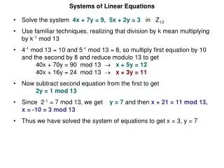
Systems of Linear Equations. Direct Methods. Solving Linear Equations. Two simultaneous equations – the solution is the intersection of two straight lines . Three simultaneous equations – the solution is the point where three planes intersect.

E N D
Systems of Linear Equations Direct Methods
Solving Linear Equations Two simultaneous equations – the solution is the intersection of two straight lines. Three simultaneous equations – the solution is the point where three planes intersect.
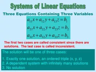
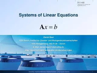
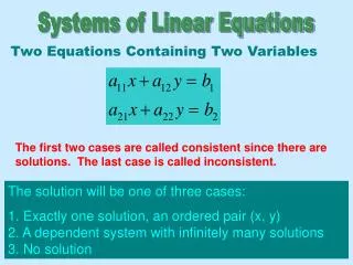
The solution of n simultaneous linear equations with n unknowns In matrix notation Ax = b, when The linear system is said to be of order n and has a unique solution if det(A) ≠ 0.
Two approaches for solving systems of linear equations • Direct Methods • Assuming negligible computational round-off errors, direct methods solve a system of linear equations in a finite number of operations. • These direct techniques are useful when the number of equations involved is not too large (typically of the order of 40 or fewer equations). • Examples of direct methods: Gauss Elimination and Gauss-Jordan Elimination.
Two approaches for solving systems of linear equations • Iterative Methods • These iterative methods are more appropriate when the number of equations involved is large (typically of the order of 100 or more), or when the matrix is sparse. • They are more economical in memory requirements. • Examples of iterative methods: Jacobi method and Gauss Seidel iterative methods
Direct Methods • Gauss Elimination • Naïve Gauss Eliminiation • Pivoting Strategies • Scaling • Gauss-Jordan Elimination • LU Decomposition
Gauss Elimination Linear systems of equations where the matrix is triangular are particularly easy to solve.
Exercise What are the values of x1, x2, x3, and x4?
Gauss Elimination Two steps of the Gaussian Elimination Forward Elimination – To transform the set of equations to an upper triangular system. Back Substitution – To find the values of x's.
Naive Gauss Elimination It is called "Naïve" Gauss Elimination because it does not avoid the problem of division by zero. Forward Elimination Purpose: to reduce the set of equations to an upper triangular system
Forward Elimination Step 1: Remove x1 from all equations except the first equation (which serves as the pivot equation.) Let's focus on removing x1 from (row 2) first.
Note:a11 is called the pivot coefficient. Forward Elimination If a11≠ 0, define m21 =a21 / a11. We can replace (row2) by {(row2) – m21 x (row1)}to yield Put We have (row 3') can be obtained in the similar fashion.
Forward Elimination After step 1, we have Step 2: Remove x2 from all equations except the first two equations (row 1) and (row 2'). That is (Basically repeat step 1 on the subsystem.)
Forward Elimination If a'22≠ 0, define m32 =a'32 / a'22. We can replace (row 3') by {(row 3') – m32 x (row 2')} to yield Put We have
Exercise What are the values of a'22, a'23, a'32, a'33, b'2, b'3 ?
Exercise (continue) What are the values of a"33 and b"33 ?
Exercise (continue) What are the values of x1, x2, x3?
Forward Elimination In general, given a linear system of n equations, we repeat the procedure until the system has been transformed into an upper triangular system.
Back Substitution After reducing the system of equations into an upper triangular system, we can start solving for x'sin backward manner.
Pseudocode to performForward Elimination for k = 1 to n-1 for i = k+1 to n factor = aik / akk for j = k+1 to n aij = aij – factor * akj bi = bi – factor * bk m21 =a21 / a11
Pseudocode to performBack Substitution xn = bn / ann for i = n-1 downto 1 sum = 0 for j = i+1 to n sum = sum + aij * xj xi = (bi – sum) / aii
Operation Count The execution time of Gauss Elimination is measured in terms of floating-point operations (FLOPS).
Operation Count (Forward Elimination) Note: for k = 1 to n-1 for i = k+1 to n factor = aik / akk for j = k+1 to n aij = aij – factor * akj bi = bi – factor * bk
Operation Count (Back Substitution) xn = bn / ann for i = n-1 downto 1 sum = 0 for j = i+1 to n sum = sum + aij * xj xi = (bi – sum) / aii
Total Number of FLOPS • Addition/Subtraction • Multiplication/Division
Total Number of FLOPS • Total number of FLOPS – O(n3) • For large n, the operation count for Gauss Elimination is about n3. This means that as n doubled, the cost of solving the linear equations goes up by a factor of 8. • It is also easy to see that most of the cost of Gauss Elimination is in the elimination step.
Direct Methods • Gauss Elimination • Naïve Gauss Eliminiation • Pivoting Strategies • Scaling • Gauss-Jordan Elimination • LU Decomposition
Pitfalls of Elimination Methods • Division by zero • When the pivot coefficient is equal to or close to zero. Example: • Round-off error • Round-off error propagates significantly when we calculate the solution of a large number of equations. • Ill-conditioned system • When the determinant is close to zero
Cases that cause problem • Singular (no solution) • Singular (infinite solution) • Ill-condition system (Near-singular)
Ill-condition System When there is a small change in one or more of the coefficients in a system, • Well condition system – results in a similar small change in the solution. • Ill-condition system – results in large changes in the solution. An example of an ill-conditioned system and its solution
Ill-condition System If we change the coefficient a21 from 1.1 to 1.05, we have the equations and the corresponding solution as Substituting the solutions back to the equations, A change of 0.05 in one of the coefficients results in a large change in the solution. However, when substituting the solutions back to the equations, we are unable to discover a large deviation.
Pivoting Strategies • Pivoting – making the magnitude of the diagonal elements (pivots) as large as possible by interchanging equations. • In Gauss Elimination, if pivot coefficient akk(k) = 0 for some k, the method breaks down. • Example: This system is non-singular and has a unique solution
However, after the 1st step in the elimination, we get x1 + x2 + x3 = 1 x3 = 1 x2 + x3 = 0 Note that a22= 0, we can't proceed as usual. But by interchanging Row 2 and Row 3, we have the triangular system x1 + x2 + x3 = 1 x2 + x3 = 0 x3 = 1
Pivoting Strategies • Partial Pivoting • Interchange equations (rows) only • Choose r, the smallest integer for which i.e. choose the largest coefficient in the column to become the pivot coefficient. • interchange rows k and r
Pivoting Strategies • Complete Pivoting • Interchange both equations and unknown elements (pivots) • Choose r and s, the smallest integer for which i.e. choose the largest coefficient in the sub-matrix to become the pivot coefficient. • interchange rows k and r, and columns k and s.
Exercise (Partial Pivoting) Suppose k = 2 (2nd iteration). Which row should be selected as the pivot row?
Exercise (Complete Pivoting) Suppose k = 2 (2nd iteration). Which row should be selected as the pivot row?
Example (Without partial pivoting) • Use Gauss elimination to solve (Ans: x1 = 1/3, x2 = 2/3) • Note that the first pivoting element a11 is close to 0. • Forward elimination gives • Backward substitution gives
(Ans: x1 = 1/3, x2 = 2/3) Error! The solution is sensitive to the number of significant figures in the computation, since we are subtracting two almost equal numbers.
Example (With partial pivoting) • Reverse order (Ans: x1 = 1/3, x2 = 2/3) • Forward elimination gives • Backward substitution gives
(Ans: x1 = 1/3, x2 = 2/3) Error! The solution is less sensitive to the number of significant figures in the computation.
Singularity x1 + x2 + x3 = 4 2x1 – x2 – x3 = 7 x1 – 2x2 – 2x3 = 12 • Now consider x1 + x2 + x3 = 4 – 3x2 – 3x3 = -1 – 3x2 – 3x3 = 8 x1 + x2 + x3 = 4 – 3x2 – 3x3 = -1 0x3 = 9 We can detect singularity during the elimination process.
Summary of Pivoting • How to perform partial and complete pivoting • Reasons for performing pivoting • Avoid division by zero • Minimize the effect of rounding error
Direct Methods • Gauss Elimination • Naïve Gauss Eliminiation • Pivoting Strategies • Scaling • Gauss-Jordan Elimination • LU Decomposition
Scaling Rescale all coefficients in a row to make the largest coefficient equal to 1. Example:
Questions • What is the effect of scaling? • What do we need to scale?
Example of Scaling • Use Gauss Elimination to solve (Ans: x1 = 1.00002, x2 = 0.99998)
Example of Scaling (Assume 3 significant digits) • Solution (a): Without pivoting and scaling • Forward elimination gives • Back substitution gives x2 = 1.00, x1 = 1.00 (Right)
Example of Scaling (Assume 3 significant digits) • Solution (b): With partial pivoting but no scaling • Forward elimination gives • Back substitution gives x2 = 1.00, x1 = 0.00 (Wrong)
Example of Scaling (Assume 3 significant digits) • Solution (c): With partial pivoting and scaling • Forward elimination gives • Back substitution gives x2 = 1.00, x1 = 1.00 (Right)