Download
1 / 53
560 likes | 817 Vues
A STOCHASTIC VARIATIONAL MULTISCALE METHOD FOR DIFFUSION IN HETEROGENEOUS RANDOM MEDIA. N. ZABARAS AND B. VELAMUR ASOKAN. Materials Process Design and Control Laboratory Sibley School of Mechanical and Aerospace Engineering 188 Frank H. T. Rhodes Hall Cornell University Ithaca, NY 14853-3801

E N D
A STOCHASTIC VARIATIONAL MULTISCALE METHOD FOR DIFFUSION IN HETEROGENEOUS RANDOM MEDIA N. ZABARAS AND B. VELAMUR ASOKAN Materials Process Design and Control Laboratory Sibley School of Mechanical and Aerospace Engineering188 Frank H. T. Rhodes Hall Cornell University Ithaca, NY 14853-3801 Email: zabaras@cornell.edu URL: http://mpdc.mae.cornell.edu/
WHY UNCERTAINTY AND MULTISCALING ? • Uncertainties introduced across various length scales have a non-trivial interaction • Current sophistications – resolve macro uncertainties Micro Meso Macro • Imprecise boundary conditions • Initial perturbations • Use micro averaged models for resolving physical scales • Physical properties, structure follow a statistical description
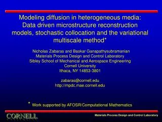
EXAMPLE 2: DIFFUSION IN A RANDOM MICROSTRUCTURE • DIFFUSION COEFFICIENTS OF INDIVIDUAL CONSTITUENTS NOT KNOWN EXACTLY • A MIXTURE MODEL IS USED THE INTENSITY OF THE GRAY-SCALE IMAGE IS MAPPED TO THE CONCENTRATIONS DARKEST DENOTES b PHASE LIGHTEST DENOTES a PHASE
OUTLINE • Motivation: coupling multiscaling and uncertainty analysis • Mathematical representation of uncertainty • Variational multiscale method (VMS) • Application of VMS with explicit subgrid model • Stochastic multiscale diffusion equation • Increasing efficiency in uncertainty modeling techniques • Sparse grid quadrature, support-space method • Future directions
UNCERTAINTY ANALYSIS TECHNIQUES • Monte-Carlo : Simple to implement, computationally expensive • Perturbation, Neumann expansions : Limited to small fluctuations, tedious for higher order statistics • Sensitivity analysis, method of moments : Probabilistic information is indirect, small fluctuations • Spectral stochastic uncertainty representation • Basis in probability and functional analysis • Can address second order stochastic processes • Can handle large fluctuations, derivations are general
RANDOM VARIABLES = FUNCTIONS ? • Math: Probability space (W, F, P) Sample space Probability measure Sigma-algebra • Random variable • : Random variable • A stochastic process is a random field with variations across space and time
SPECTRAL STOCHASTIC REPRESENTATION • A stochastic process = spatially, temporally varying random function CHOOSE APPROPRIATE BASIS FOR THE PROBABILITY SPACE GENERALIZED POLYNOMIAL CHAOS EXPANSION HYPERGEOMETRIC ASKEY POLYNOMIALS SUPPORT-SPACE REPRESENTATION PIECEWISE POLYNOMIALS (FE TYPE) KARHUNEN-LOÈVE EXPANSION SPECTRAL DECOMPOSITION SMOLYAK QUADRATURE, CUBATURE, LH COLLOCATION, MC (DELTA FUNCTIONS)
KARHUNEN-LOEVE EXPANSION ON random variables Mean function Stochastic process Deterministic functions • Deterministic functions ~ eigen-values , eigenvectors of the covariance function • Orthonormal random variables ~ type of stochastic process • In practice, we truncate (KL) to first N terms
GENERALIZED POLYNOMIAL CHAOS • Generalized polynomial chaos expansion is used to represent the stochastic output in terms of the input Stochastic input Askey polynomials in input Stochastic output Deterministic functions • Askey polynomials ~ type of input stochastic process • Usually, Hermite, Legendre, Jacobi etc.
SUPPORT-SPACE REPRESENTATION • Any function of the inputs, thus can be represented as a function defined over the support-space FINITE ELEMENT GRID REFINED IN HIGH-DENSITY REGIONS • SMOLYAK QUADRATURE • IMPORTANCE MONTE CARLO JOINT PDF OF A TWO RANDOM VARIABLE INPUT OUTPUT REPRESENTED ALONG SPECIAL COLLOCATION POINTS
NEED FOR SUPPORT-SPACE APPROACH • GPCE and Karhunen-Loeve are Fourier like expansions • Gibb’s effect in describing highly nonlinear, discontinuous uncertainty propagation Onset of natural convection [Zabaras JCP 208(1)] – Using support-space method [Ghanem JCP 197(1)] – Using Wiener-Haar wavelets • Finite element representation of stochastic processes [stochastic Galerkin method: Babuska et al] • Incorporation of importance based meshing concept for improving accuracy [support space method]
CURSE OF DIMENSIONALITY • Both GPCE and support-space method are fraught with the curse of dimensionality • As the number of random input orthonormal variables increase, computation time increases exponentially • Support-space grid is usually in a higher-dimensional manifold (if the number of inputs is > 3), we need special tensor product techniques for generation of the support-space • Parallel implementations are currently performed using PETSc (Parallel scientific extensible toolkit )
Actual solution Subgrid scale solution Coarse scale solution h VARIATIONAL MULTISCALE METHOD Hypothesis • Exact solution = Coarse resolved part + Subgrid part [Hughes, 95, CMAME] Induced function space • Solution function space = Coarse function space + Subgrid function space Idea • Model the projection of weak form onto the subgrid function space, calculate an approximate subgrid solution • Use the subgrid solution to solve for coarse solution
VARIATIONAL MULTISCALE BASICS DERIVE THE WEAK FORMULATION FOR THE GOVERNING EQUATIONS PROJECT THE WEAK FORMULATION ON COARSE AND FINE SCALES SOLUTION FUNCTION SPACES ARE NOW STOCHASTIC FUNCTION SPACES COARSE WEAK FORM FINE (SUBGRID) WEAK FORM ALGEBRAIC SUBGRID MODELS COMPUTATIONAL SUBGRID MODELS REMOVE SUBGRID EFFECTS IN THE COARSE WEAK FORM USING STATIC CONDENSATION APPROXIMATE SUBGRID SOLUTION NEED TECHNIQUES TO SOLVE STOCHASTIC PDEs MODIFIED MULTISCALE COARSE WEAK FORM INCLUDING SUBGRID EFFECTS
FINAL COARSE FORMULATION VMS HYPOTHESIS AFFINE CORRECTION DERIVE WEAK FORM COARSE-TO-SUBGRID MAP DEFINE PROBLEM MODEL MULTISCALE HEAT EQUATION in on in THE DIFFUSION COEFFICIENT K IS HETEROGENEOUS AND POSSESSES RAPID RANDOM VARIATIONS IN SPACE • OTHER APPLICATIONS • DIFFUSION IN COMPOSITES • FUNCTIONALLY GRADED MATERIALS FLOW IN HETEROGENEOUS POROUS MEDIA INHERENTLY STATISTICAL DIFFUSION IN MICROSTRUCTURES
FINAL COARSE FORMULATION VMS HYPOTHESIS AFFINE CORRECTION DERIVE WEAK FORM COARSE-TO-SUBGRID MAP DEFINE PROBLEM STOCHASTIC WEAK FORM such that, for all : Find • Weak formulation • VMS hypothesis Exact solution Subgrid solution Coarse solution
EXPLICIT SUBGRID MODELLING: IDEA DERIVE THE WEAK FORMULATION FOR THE GOVERNING EQUATIONS PROJECT THE WEAK FORMULATION ON COARSE AND FINE SCALES COARSE WEAK FORM FINE (SUBGRID) WEAK FORM COARSE-TO-SUBGRID MAP EFFECT OF COARSE SOLUTION ON SUBGRID SOLUTION AFFINE CORRECTION SUBGRID DYNAMICS THAT ARE INDEPENDENT OF THE COARSE SCALE LOCALIZATION, SOLUTION OF SUBGRID EQUATIONS NUMERICALLY FINAL COARSE WEAK FORMULATION THAT ACCOUNTS FOR THE SUBGRID SCALE EFFECTS
FINAL COARSE FORMULATION VMS HYPOTHESIS AFFINE CORRECTION DERIVE WEAK FORM COARSE-TO-SUBGRID MAP DEFINE PROBLEM SCALE PROJECTION OF WEAK FORM such that, for all Find and and • Projection of weak form on coarse scale • Projection of weak form on subgrid scale EXACT SUBGRID SOLUTION COARSE-TO-SUBGRID MAP SUBGRID AFFINE CORRECTION
SPLITTING THE SUBGRID SCALE WEAK FORM • Subgrid scale weak form • Coarse-to-subgrid map • Subgrid affine correction
NATURE OF MULTISCALE DYNAMICS ASSUMPTIONS: NUMERICAL ALGORITHM FOR SOLUTION OF THE MULTISCALE PDE COARSE TIME STEP SUBGRID TIME STEP 1 1 ũC ūC Coarse solution field at end of time step Coarse solution field at start of time step ûF
REPRESENTING COARSE SOLUTION ELEMENT COARSE MESH RANDOM FIELD DEFINED OVER THE ELEMENT FINITE ELEMENT PIECEWISE POLYNOMIAL REPRESENTATION USE GPCE TO REPRESENT THE RANDOM COEFFICIENTS • Given the coefficients , the coarse scale solution is completely defined
FINAL COARSE FORMULATION VMS HYPOTHESIS AFFINE CORRECTION DERIVE WEAK FORM COARSE-TO-SUBGRID MAP DEFINE PROBLEM COARSE-TO-SUBGRID MAP ELEMENT COARSE MESH ANY INFORMATION FROM COARSE TO SUBGRID SOLUTION CAN BE PASSED ONLY THROUGH BASIS FUNCTIONS THAT ACCOUNT FOR FINE SCALE EFFECTS INFORMATION FROM COARSE SCALE COARSE-TO-SUBGRID MAP
SOLVING FOR THE COARSE-TO-SUBGRID MAP START WITH THE WEAK FORM APPLY THE MODELS FOR COARSE SOLUTION AND THE C2S MAP AFTER SOME ASSUMPTIONS ON TIME STEPPING THIS IS DEFINED OVER EACH ELEMENT, IN EACH COARSE TIME STEP
BCs FOR THE COARSE-TO-SUBGRID MAP INTRODUCE A SUBSTITUTION CONSIDER AN ELEMENT
FINAL COARSE FORMULATION VMS HYPOTHESIS AFFINE CORRECTION DERIVE WEAK FORM COARSE-TO-SUBGRID MAP DEFINE PROBLEM SOLVING FOR SUBGRID AFFINE CORRECTION START WITH THE WEAK FORM • WHAT DOES AFFINE CORRECTION MODEL? • EFFECTS OF SOURCES ON SUBGRID SCALE • EFFECTS OF INITIAL CONDITIONS CONSIDER AN ELEMENT IN A DIFFUSIVE EQUATION, THE EFFECT OF INITIAL CONDITIONS DECAY WITH TIME. WE CHOOSE A CUT-OFF • To reduce cut-off effects and to increase efficiency, we can use the quasistatic subgrid assumption
COMPUTATIONAL ISSUES • Based on the indices in the C2S map and the affine correction, we need to solve (P+1)(nbf) problems in each coarse element • At a closer look we can find that • This implies, we just need to solve (nbf) problems in each coarse element (one for each index s)
FINAL COARSE FORMULATION VMS HYPOTHESIS AFFINE CORRECTION DERIVE WEAK FORM COARSE-TO-SUBGRID MAP DEFINE PROBLEM MODIFIED COARSE SCALE FORMULATION • We can substitute the subgrid results in the coarse scale variational formulation to obtain the following • We notice that the affine correction term appears as an anti-diffusive correction • Often, the last term involves computations at fine scale time steps and hence is ignored
NUMERICAL EXAMPLES • Stochastic investigations • Example 1: Decay of a sine hill in a medium with random diffusion coefficient • The diffusion coefficient has scale separation and periodicity • Example 2: Planar diffusion in microstructures • The diffusion coefficient is computed from a microstructure image • The properties of microstructure phases are not known precisely [source of uncertainty] • Future issues
QUASISTATIC SEEMS BETTER • There are two important modeling considerations that were neglected for the dynamic subgrid model • Effect of the subgrid component of the initial conditions on the evolution of the reconstructed fine scale solution • Better models for the initial condition specified for the C2S map (currently, at time zero, the C2S map is identically equal to zero implying a completely coarse scale formulation) • In order to avoid the effects of C2S map, we only store the subgrid basis functions beyond a particular time cut-off (referred to herein as the burn-in time) • These modeling issues need to be resolved for increasing the accuracy of the dynamic subgrid model
EXAMPLE 2: DIFFUSION IN A RANDOM MICROSTRUCTURE • DIFFUSION COEFFICIENTS OF INDIVIDUAL CONSTITUENTS NOT KNOWN EXACTLY • A MIXTURE MODEL IS USED THE INTENSITY OF THE GRAY-SCALE IMAGE IS MAPPED TO THE CONCENTRATIONS DARKEST DENOTES b PHASE LIGHTEST DENOTES a PHASE
RESULTS AT TIME = 0.05 FIRST ORDER GPCE COEFF MEAN SECOND ORDER GPCE COEFF RECONSTRUCTED FINE SCALE SOLUTION (VMS) FULLY RESOLVED GPCE SIMULATION
RESULTS AT TIME = 0.2 FIRST ORDER GPCE COEFF MEAN SECOND ORDER GPCE COEFF RECONSTRUCTED FINE SCALE SOLUTION (VMS) FULLY RESOLVED GPCE SIMULATION
HIGHER ORDER TERMS AT TIME = 0.2 FOURTH ORDER GPCE COEFF THIRD ORDER GPCE COEFF FIFTH ORDER GPCE COEFF RECONSTRUCTED FINE SCALE SOLUTION (VMS) FULLY RESOLVED GPCE SIMULATION
UNCERTAINTY RELATED • THE EXAMPLES USED ASSUME A CORRELATION FUNCTION FOR INPUTS, USE KARHUNEN-LOEVE EXPANSION GPCE (OR) SUPPORT-SPACE • PHYSICAL ASPECTS OF AN UNCERTAINTY MODEL, DERIVATION OF CORRELATION, DISCTRIBUTIONS USING EXPERIMENTS AND SIMULATION ROUGHNESS PERMEABILITY • AVAILABLE GAPPY DATA • BAYESIAN INFERENCE • WHAT ABOUT THE MULTISCALE NATURE ? • BOTH GPCE AND SUPPORT-SPACE ARE SUCCEPTIBLE TO CURSE OF DIMENSIONALITY • USE OF SPARSE GRID QUADRATURE SCHEMES FOR HIGHER DIMENSIONS (SMOLYAK, GESSLER, XIU) • FOR VERY HIGH DIMENSIONAL INPUT, USING MC ADAPTED WITH SUPPORT-SPACE, GPCE TECHNIQUES
SPARSE GRID QUADRATURE • If the number of random inputs is large (dimension D ~ 10 or higher), the number of grid points to represent an output on the support-space mesh increases exponentially • GPCE for very high dimensions yields highly coupled equations and ill-conditioned systems (relative magnitude of coefficients can be drastically different) • Instead of relying on piecewise interpolation, series representations, can we choose collocation points that still ensure accurate interpolations of the output (solution)
SMOLYAK ALGORITHM LET OUR BASIC 1D INTERPOLATION SCHEME BE SUMMARIZED AS IN MULTIPLE DIMENSIONS, THIS CAN BE WRITTEN AS TO REDUCE THE NUMBER OF SUPPORT NODES WHILE MAINTAINING ACCURACY WITHIN A LOGARITHMIC FACTOR, WE USE SMOLYAK METHOD IDEA IS TO CONSTRUCT AN EXPANDING SUBSPACE OF COLLOCATION POINTS THAT CAN REPRESENT PROGRESSIVELY HIGHER ORDER POLYNOMIALS IN MULTIPLE DIMENSIONS A FEW FAMOUS SPARSE QUADRATURE SCHEMES ARE AS FOLLOWS: CLENSHAW CURTIS SCHEME, MAXIMUM-NORM BASED SPARSE GRID AND CHEBYSHEV-GAUSS SCHEME
SPARSE GRID COLLOCATION METHOD Solution Methodology PREPROCESSING Compute list of collocation points based on number of stochastic dimensions, N and level of interpolation, q Compute the weighted integrals of all the interpolations functions across the stochastic space (wi) Use any validated deterministic solution procedure. Completely non intrusive Solve the deterministic problem defined by each set of collocated points POSTPROCESSING Compute moments and other statistics with simple operations of the deterministic data at the collocated points and the preprocessed list of weights Std deviation of temperature: Natural convection
USING THE COLLOCATION METHOD FOR HIGHER DIMENSIONS • Flow through heterogeneous random media Alloy solidification, thermal insulation, petroleum prospecting Look at natural convection through a realistic sample of heterogeneous material Square cavity with free fluid in the middle part of the domain. The porosity of the material is taken from experimental data1 Left wall kept heated, right wall cooled Numerical solution procedure for the deterministic procedure is a fractional time stepping method 1. Reconstruction of random media using Monte Carlo methods, Manwat and Hilfer, Physical Review E. 59 (1999)
FLOW THROUGH HETEROGENEOUS RANDOM MEDIA Experimental correlation for the porosity of the sandstone. Eigen spectrum is peaked. Requires large dimensions to accurately represent the stochastic space Simulated with N= 20 Number of collocation points is 11561 (level 4 interpolation) Material: Sandstone Numerically computed Eigen spectrum
FLOW THROUGH HETEROGENEOUS RANDOM MEDIA FIRST MOMENT Snapshots at a few collocation points Temperature y-Velocity Temperature Y velocity Streamlines SECOND MOMENT Temperature Y velocity
USING THE COLLOCATION METHOD FOR HIGHER DIMENSIONS 2. Flow over rough surfaces Thermal transport across rough surfaces, heat exchangers Look at natural convection through a realistic roughness profile Rectangular cavity filled with fluid. Lower surface is rough. Roughness auto correlation function from experimental data2 Lower surface maintained at a higher temperature Rayleigh-Benard instability causes convection Numerical solution procedure for the deterministic procedure is a fractional time stepping method T (y) = -0.5 T (y) = 0.5 y = f(x,ω) 2. H. Li, K. E. Torrance, An experimental study of the correlation between surface roughness and light scattering for rough metallic surfaces, Advanced Characterization Techniques for Optics, Semiconductors, and Nanotechnologies II,
NATURAL CONVECTION ON ROUGH SURFACES Experimental ACF Experimental correlation for the surface roughness Eigen spectrum is peaked. Requires large dimensions to accurately represent the stochastic space Simulated with N= 20 (Represents 94% of the spectrum) Number of collocation points is 11561 (level 4 interpolation) Numerically computed Eigen spectrum Sample realizations of temperature at collocation points
NATURAL CONVECTION ON ROUGH SURFACES FIRST MOMENT SECOND MOMENT Temperature Temperature Streamlines Y Velocity Roughness causes improved thermal transport due to enhanced nonlinearities Results in thermal plumes Can look to tailor material surfaces to achieve specific thermal transport
PROBLEM DEFINITION We have a class of microstructures which share certain features between each other. We want to compute statistical variability of certain diffusion related fields, such as temperature, within this class of microstructures. The variability in the microstructural class is due to variations in grain sizes. SUB PROBLEMS • 1. How do you compute the class of microstructures? • - MaxEnt • 2. How do you interrogate this class of microstructures for diffusion problems? • - Stochastic collocation schemes • 3. How do you compute microstructures at collocation points? • - POD method