2D Transformations
Understand 2D transformations - translation, rotation, scaling - and how to apply matrix operations to objects. Learn about point representation, matrices for translation and rotation, and scaling techniques.

2D Transformations
E N D
Presentation Transcript
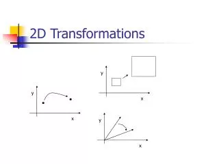
2D Transformations y y x x y x
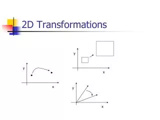
2D Transformation • Given a 2D object, transformation is to change the object’s • Position (translation) • Size (scaling) • Orientation (rotation) • Shapes (shear) • Apply a sequence of matrix multiplication to the object vertices
X’ a b c x Y’ = d e f * y 1 0 0 1 1 Point representation • We can use a column vector (a 2x1 matrix) to represent a 2D point x y • A general form of linear transformation can be written as: x’ = ax + by + c OR y’ = dx + ey + f
(x’,y’) (x,y) Translation • Re-position a point along a straight line • Given a point (x,y), and the translation distance (tx,ty) The new point: (x’, y’) x’ = x + tx y’ = y + ty ty tx OR P’ = P + T where P’ = x’ p = x T = tx y’ y ty
x’ = x + tx y’ y ty x’ 1 0 tx x y’ = 0 1 ty * y 1 0 0 1 1 3x3 2D Translation Matrix Use 3 x 1 vector • Note that now it becomes a matrix-vector multiplication
Translate individual vertices Translation • How to translate an object with multiple vertices?
q 2D Rotation • Default rotation center: Origin (0,0) • > 0 : Rotate counter clockwise q • < 0 : Rotate clockwise
(x’,y’) (x’, y’) q f (x,y) Rotation (x,y) -> Rotate about the origin by q r How to compute (x’, y’) ? x = r cos (f)y = r sin (f) x’ = r cos (f + q)y = r sin (f + q)
(x’,y’) q f (x,y) Rotation x = r cos (f)y = r sin (f) x’ = r cos (f + q)y = r sin (f + q) r x’ = r cos (f + q) = r cos(f) cos(q) – r sin(f) sin(q) = x cos(q) – y sin(q) y’ = r sin (f + q) = r sin(f) cos(q) + r cos(f)sin(q) = y cos(q) + x sin(q)
(x’,y’) q f x’ cos(q) -sin(q) x y’ sin(q) cos(q) y = (x,y) Rotation x’ = x cos(q) – y sin(q) y’ = y cos(q) + x sin(q) r Matrix form? 3 x 3?
(x’,y’) r q f x’ cos(q) -sin(q) 0 x y’ sin(q) cos(q) 0 y 1 0 0 1 1 x’ cos(q) -sin(q) x y’ sin(q) cos(q) y = = (x,y) 3x3 2D Rotation Matrix
q Rotate individual Vertices Rotation • How to rotate an object with multiple vertices?
x’ Sx 0 x y’ 0 Sy y x’ = x . Sx y’ = y . Sy = (4,4) Sx = 2, Sy = 2 (2,2) (2,2) (1,1) 2D Scaling Scale: Alter the size of an object by a scaling factor (Sx, Sy), i.e.
(4,4) Sx = 2, Sy = 2 (2,2) (2,2) (1,1) 2D Scaling • Not only the object size is changed, it also moved!! • Usually this is an undesirable effect • We will discuss later (soon) how to fix it
x’ Sx 0 x y’ 0 Sy y = x’ Sx 0 0 x y’ = 0 Sy 0 * y 1 0 0 1 1 3x3 2D Scaling Matrix
Put it all together • Translation: x’ x tx y’ y ty • Rotation: x’ cos(q) -sin(q) x y’ sin(q) cos(q) y • Scaling: x’ Sx 0 x y’ 0 Sy y = + = * = *
x’ 1 0 tx x y’ = 0 1 ty * y 1 0 0 1 1 Or, 3x3 Matrix representations • Translation: • Rotation: • Scaling: Why use 3x3 matrices? x’ cos(q) -sin(q) 0 x y’ sin(q) cos(q) 0 * y 1 0 0 1 1 = x’ Sx 0 0 x y’ = 0 Sy 0 * y 1 0 0 1 1
Why use 3x3 matrices? • So that we can perform all transformations using matrix/vector multiplications • This allows us to pre-multiply all the matrices together • The point (x,y) needs to be represented as (x,y,1) -> this is called Homogeneous coordinates!
x 1 h 0 x y = 0 1 0 * y 1 0 0 1 1 Shearing • Y coordinates are unaffected, but x cordinates are translated linearly with y • That is: • y’ = y • x’ = x + y * h
Interesting Facts: • A 2D rotation is three shears • Shearing will not change the area of the object • Any 2D shearing can be done by a rotation, followed by a scaling, and followed by a rotation x 1 0 0 x y = g 1 0 * y 1 0 0 1 1 Shearing in y
What if I want to rotate about an arbitrary center? Rotation Revisit • The standard rotation matrix is used to rotate about the origin (0,0) cos(q) -sin(q) 0 sin(q) cos(q) 0 0 0 1
(px,py) Arbitrary Rotation Center • To rotate about an arbitrary point P (px,py) by q: • Translate the object so that P will coincide with the origin: T(-px, -py) • Rotate the object: R(q) • Translate the object back: T(px,py)
x’ 1 0 px cos(q) -sin(q) 0 1 0 -px x y’ = 0 1 py sin(q) cos(q) 0 0 1 -py y 1 0 0 1 0 0 1 0 0 1 1 Arbitrary Rotation Center • Translate the object so that P will coincide with the origin: T(-px, -py) • Rotate the object: R(q) • Translate the object back: T(px,py) • Put in matrix form: T(px,py) R(q) T(-px, -py) * P
What if I want to scale about an arbitrary pivot point? Scaling Revisit • The standard scaling matrix will only anchor at (0,0) Sx 0 0 0 Sy 0 0 0 1
Arbitrary Scaling Pivot • To scale about an arbitrary pivot point P (px,py): • Translate the object so that P will coincide with the origin: T(-px, -py) • Rotate the object: S(sx, sy) • Translate the object back: T(px,py) (px,py)
Affine Transformation • Translation, Scaling, Rotation, Shearing are all affine transformation • Affine transformation – transformed point P’ (x’,y’) is a linear combination of the original point P (x,y), i.e. x’ m11 m12 m13 x y’ = m21 m22 m23 y 1 0 0 1 1 • Any 2D affine transformation can be decomposed into a rotation, followed by a scaling, followed by a shearing, and followed by a translation. Affine matrix = translation x shearing x scaling x rotation
(pre-multiply) M Composing Transformation • Composing Transformation – the process of applying several transformation in succession to form one overall transformation • If we apply transform a point P using M1 matrix first, and then transform using M2, and then M3, then we have: (M3 x (M2 x (M1 x P ))) = M3 x M2 x M1 x P
Composing Transformation • Matrix multiplication is associative M3 x M2 x M1 = (M3 x M2) x M1 = M3 x (M2 x M1) • Transformation products may not be commutative A x B != B x A • Some cases where A x B = B x A A B translation translation scaling scaling rotation rotation uniform scaling rotation (sx = sy)
Transformation order matters! • Example: rotation and translation are not commutative Translate (5,0) and then Rotate 60 degree OR Rotate 60 degree and then translate (5,0)?? Rotate and then translate !!
How OpenGL does it? • OpenGL’s transformation functions are meant to be used in 3D • No problem for 2D though – just ignore the z dimension • Translation: • glTranslatef(d)(tx, ty, tz) -> glTranslatef(d)tx,ty,0) for 2D
y x z How OpenGL does it? • Rotation: • glRotatef(d)(angle, vx, vy, vz) -> glRotatef(d)(angle, 0,0,1) for 2D y (vx, vy, vz) – rotation axis x You can imagine z is pointing out of the slide
OpenGL Transformation Composition • A global modeling transformation matrix (GL_MODELVIEW, called it M here) glMatrixMode(GL_MODELVIEW) • The useris responsible to reset it if necessary glLoadIdentity() -> M = 1 0 0 0 1 0 0 0 1
OpenGL Transformation Composition • Matrices for performing user-specified transformations are multiplied to the model view global matrix • For example, 1 0 1 glTranslated(1,1 0); M = M x 0 1 1 0 0 1 • All the vertices P defined within glBegin() will first go through the transformation (modeling transformation) P’ = M x P
Object Local Coordinates Object World Coordinates Transformation Pipeline Modeling transformation …


