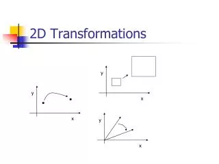
Transformations and viewing in 2D
2D Transformations. TranslationRotationScalingReflectionOthers. 2D Transformations, cont'd. A new point (x', y') shall be generated from an existing point (x, y)Actually, only points are transformed!E.g. * for a line - the two endpoints* for a polygon - the vertices* for a circle - the m

Transformations and viewing in 2D
E N D
Presentation Transcript
1. Transformations and viewing in 2D 2D transformations
Windows and viewports
Clipping
2. 2D Transformations Translation
Rotation
Scaling
Reflection
Others
3. 2D Transformations, cont�d A new point (x�, y�) shall be generated from an existing point (x, y)
Actually, only points are transformed!
E.g.
* for a line - the two endpoints
* for a polygon - the vertices
* for a circle - the midpoint
4. Translation If Tx and Ty corresponds to the relative movements in the two main directions, then
x� = x + Tx
y� = y + Ty
5. Rotation Additional specifications are required, e.g.
rotation relative to origin
an angle of rotation, ?
counterclockwise (or clockwise)
Then
x� = x.cos ? - y.sin ?
y� = x.sin ? + y.cos ?
6. Scaling Additional requirement:
scaling relative to origin
Then
x� = x.Sx
y� = y.Sy
Note! Sx and Sy are typically the same.
7. 2D Transformations, cont�d A sequence of transformations can be combined into one transformation.
Then, the order is important
Often more convienient to use matrix representation of the transformations, especially if they are going to be combined.
8. Homogeneous Coordinate System Any 2D transformation can be described uniquely by a 3x3 matrix, if the Cartesian coordinates (x, y) is represented by the homogeneous coordinate triple (xw, yw, w),
where x=xw/w, y=yw/w and w can be any real value ? 0, for simplicity w=1 is used here
9. Homogeneous Matrix Representation
Then, the transformation
(x, y) => (x�, y�)
is generally represented by
10. Translation Matrix Moving Tx in x-direction and Ty in y-direction:
11. Rotation Matrix Rotate ? degrees about origin in counter-clockwise direction:
12. Scaling Matrix Scaling with factors Sx and Sy relative to origin:
13. Combining simple transformations More complex transformations can be combined and expressed by using one single 3x3 matrix, which is the product of all the combined simple matrices.
Note! The order between the matrices is crucial!
14. Example with a combined transformation A point (x, y) shall be rotated ? degrees in clockwise direction about the point (Rx,Ry).
Three steps:
1) Move (Rx, Ry) to origin
2) Rotate ? degrees about origin
3) Move back to (Rx, Ry)
15. Example, step 1)
16. Example, step 2)
17. Example, step 3)
18. Example, result
19. Scaling Example Also scaling can be done relative to an arbitrary point (Rx, Ry):
20. Some reflection matrices
21. Viewing in 2D Generally, an image is defined in a world coordinate system, WC
To restrict the image in WC a window is defined, typically of rectangular shape
a) The process to transform the window (in WC) to a viewport in device coordinates is called the viewing transformation. Also, local viewport coordinates (VC) can be used within the viewport.
22. Viewing in 2D, cont�d b) The process to eliminate image parts outside the window is called clipping.
23. Viewing Transformation For a point (xw,yw) in the window to have the same relative position in the viewport, (xv,yv), the following conditions have to be fulfilled (proportionality rules):
24. Viewing Coordinates
25. Clipping When specifying a window some parts of the image are inside the window (visible) and some are not (invisible).
Clipping: a process that divides each element of an image in its visible and invisible parts, and then throw away the invisible ones.
26. Clipping different objects Point clipping
A point (x,y) is visible if
xmin=x=xmax and ymin=y=ymax
Line clipping
Polygon clipping
Curve clipping
Text clipping
27. Line Clipping Too time consuming to check each point of a line; larger parts of the line must be clipped in each step
28. Cohen-Sutherland�s Line Clipping Algorithm Main idea: At most one visible part per line (if a rectangular window) means that it�s enough to decide the two endpoints of the visible part.
Extend the edges of the window giving 9 regions with a unique 4-bit code related to each of them, where
Bit 1 corresponds to Top
Bit 2 corresponds to Bottom
Bit 3 corresponds to Right
Bit 4 corresponds to Left
29. Algorithm, cont�d The endpoints of each line are then assigned a code corresponding to the region to which they belong
30. Algorithm, cont�d The following three steps are then repeated for each line:
if the codes for both endpoints are equal to zero (0000)=> the line is inside the window (visible)
if the logical intersection (AND) between the endpoint codes is not equal to zero => the whole line is outside (invisible)
31. Algorithm, cont�d 3) else divide the line at an intersection with a window edge (or its extension!) and throw away the outside part, update the code for the new endpoint and repeat with the new line from 1)
Step 3) is done as follows
32. Algorithm, step 3) Assume endpoints (x1, y1) and (x2, y2).
The line equation can then be written:
y=y1 + k*(x - x1), k=(y2 - y1)/(x2 - x1)
When clipping against x=xmin or x=xmax, the x-coordinate of the intersection is given, and the corresponding y is then calculated from the above equation.
33. Algorithm, step 3), cont�d Correspondingly, when clipping against y=ymin and y=ymax the line equation is rewritten to calculate the x-coordinate of the intersection point:
y=y1 + k*(x - x1) => x=x1 + 1/k*(y - y1)
34. Polygon Clipping In principle, line clipping could be used to clip
polygons as well. The major problem with that
approach is to keep track of the parts belonging
to the polygon and possible polygon filling.
35. Polygon Clipping, cont�d A polygon clipping method should first
generate one or more closed areas
based on an input sequence of the
vertices of the original polygon. The
output from the clipping step is a new
sequence of vertices defining the
resulting polygon
36. Polygon Clipping, cont�d Finally, the new polygon is scan converted for
correct area fill
37. Sutherland-Hodgeman�s Polygon Clipping Algorithm Best with convex polygons.
Basic principle: Clip the polygon against one (extended!) window edge at a time
=> 4 clippers are required (one for each edge)
The initial input sequence of vertices will
then be updated successively during each
of the four clipping steps.
38. Algorithm Four possible cases are recognized when
processing the polygon vertices in
sequence around the polygon perimeter
depending on the pairwise relation
between two successive vertices:
39. Algorithm, cont�d out -> in: intersection point and second vertex -> vertex list
in -> in: second vertex -> vertex list
in -> out: intersection point -> vertex list
out -> out: nothing -> vertex list
Finally, the last and the first vertices are
connected.
40. Algorithm, cont�d Concave polygons resulting in more than one area section will have a connecting line on the window boundary!
Example (separate)
41. Curve Clipping Similar methods as for lines and polygons but more processing is required due to non-linear equations.
For a curved object a bounding rectangle can be used to make a first test for overlap.
42. Text Clipping In general, methods depend on how characters are represented
However, three strategies can be followed:
all-or-none string clipping
use a bounding rectangle for the string
all-or-none character clipping
use a bounding rectangle for the character
individual character clipping
like line/curve clipping (outlined char�s)
compare individual pixels (bit-mapped)
43. Text Clipping,examples
44. External Clipping So far, the clipping discussion has been about what is specified as internal clipping (throw away outside parts).
But also external clipping (throw away inside parts) is commonly used, e.g. in multiple-window systems which are standard in today�s GUI�s