Download
1 / 51
520 likes | 801 Vues
1587: COMMUNICATION SYSTEMS 1 Wide Area Networks. Dr. George Loukas. University of Greenwich , 2012-2013. Type of network by area covered. Metropolitan Area Network. Wide Area Network. Internet. WAN. MAN. Personal Area Network. LAN. PAN. Local Area Network. BAN. Body Area Network.

E N D
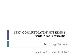
1587: COMMUNICATION SYSTEMS 1Wide Area Networks Dr. George Loukas University of Greenwich, 2012-2013
Type of network by area covered Metropolitan Area Network Wide Area Network Internet WAN MAN Personal Area Network LAN PAN Local Area Network BAN Body Area Network
Wide Area Networks Wide Area Network WAN • Use local and long-distance telecommunications • Usually very high speed with low error rates • Usually follow a mesh topology
Network Mesh A mesh is a network where all nodes can send, receive and relay data A mesh is fully connected when all nodes are directly connected to all other nodes
Fully connected Mesh 4 nodes, 6 links. Is that a problem? 8 nodes, 45 links. Is that a problem? For fully connected network: For 50 nodes, links
Fully connected Mesh: exercises 6 9 nodes and _____ links If it were a fully connected mesh, it would have ____________________ links (6 • 5)/2 =15 A network has 7 nodes. All nodes are connected with each other except for one node, which is connected to only one other node. How many links does the network have? It’s a 6-node fully connected mesh with one extra node attached to it through one link. So, 15 + 1 = 16 links.
Network Mesh A node is a device (computer, router, …) that allows the transfer of information A station is a device that interfaces a user to a network The sub-network is the connection of nodes and telecommunication links. There are three types: Message-switched Circuit-switched Packet-switched
Sub-network: Types Message-switched Circuit-switched Packet-switched Store-and-forward Good for broadcasting Today completely obsolete Example: Telex
processing + queuing delay Intermediate node 2 Intermediate node 1 Start sending first message source destination message transmission delay Finish sending first message propagation delay message source Intermediate node 2 Intermediate node 1 message destination Message-switched Circuit-switched Packet-switched
Sub-network: Types A dedicated circuit (physical path) is established between sender and receiver and all data passes over this circuit. The connection is dedicated until one party or another terminates the connection. Fixed Data Rate. Today increasingly uncommon Example: Telephone (PSTN) Message-switched Circuit-switched Packet-switched
Intermediate node 1 Intermediate node 2 source destination searching for a connection call set up acknowledgement comes back Data Message-switched Circuit-switched Packet-switched
Circuit establishment Information transfer Control Signal Data Sender node node node node Control signal node Receiver Circuit disconnection Message-switched Circuit-switched Packet-switched
Sub-network: Types All data messages are transmitted using suitably sized packages, called packets. Packets contain data and a header. No unique dedicated physical path example: Internet Two types: Datagrams and Virtual Circuits Internet Message-switched Circuit-switched Packet-switched
PACKET 1 PACKET 1 PACKET 1 PACKET 2 PACKET 2 PACKET 2 processing + queuing delay PACKET 3 PACKET 3 PACKET 3 Intermediate node 1 Intermediate node 2 source destination transmission delay propagation delay Message-switched Circuit-switched Packet-switched
Packet transfer delay = transmission + propagation + queuing + processing Depends on packet length L (bits) and link bandwidth R (bits/s). Transmission delay = L / R Depends on congestion Depends on speed of processor (for error-checking etc.) Depends on length of physical link d (m) and propagation speed is medium s (m/s). Propagation delay = d / s If the queuing delay is 4 ms, the processing delay is 1 ms, the propagation delay is insignificant, and the link bandwidth is 8 Mbps, what is the total packet transfer delay for a 1,000-byte packet over one such link? L = 1,000 bytes = 8•103 bits L / R = 10-3 s = 1 ms R = 8 Mbps = 8•106 bits/s Packet transfer delay = transmission + propagation + queuing + processing = 1 ms + 0 + 4 ms + 1 ms = 6 ms Message-switched Circuit-switched Packet-switched
Packet-switching: Datagrams Data 1 Data 2 Data 3 Datagrams Message-switched Circuit-switched Packet-switched Each packet carries extra overheads, e.g. addresses (source and destination) seq number etc.
Packet-switching: Virtual Circuit Establishing the Circuit Disconnecting the Circuit Transferring information Data 3 Data 2 Data 1 Control sender Control receiver Datagrams Virt. Circuits Message-switched Circuit-switched Packet-switched Identifier (label) Faster switching No seq number required
Packet-switching: Virtual Circuit Datagrams Virt. Circuits Message-switched Circuit-switched Packet-switched • Switched virtual circuit (SVC) • exists only for the duration of the data transfer • For each connection, a new circuit must be created • Permanent virtual circuits (PVC) • like leased lines, on a continuous basis • dedicated to specific user and no-one else can use it • no connection establishment or termination • user of a PVC will always get the same route
Circuit Switching Vs. Packet Switching Circuit switching • setup delay • no other noticeable delays Packet Switching • Virtual-circuit packet switching • setup delay • call acceptance response may experience delays • data packets are queued at each node • may experience delays - depending on load • Datagrams • no call setup • need to carry full address in each packet Datagrams Virt. Circuits Message-switched Circuit-switched Packet-switched
Circuit Switching Vs. Packet Switching CIRCUIT-Switched PACKET-Switched
Types of traffic • Stream traffic - lengthy and continuous • Bursty traffic - short sporadic transmissions Maria Lin Maria: Good morning Lin. Good morning Lin.
Network Congestion • When a part of the network has so much traffic that individual packets are delayed noticeably • Can be caused by node and link failures; high amounts of traffic; improper network planning. • Severe congestion overflows buffers and causes packet losses
Routing Each node in a WAN is a router. Multiple possible routes. How does a router decide where to route?
Routing • Every network is essentially a weighted graph of nodes and links • The links between nodes have associated costs, such as: • Delay • Number of hops • Bandwidth • Financial cost
Routing: Flooding Least intelligent, but useful sometimes • All possible routes are tried • All nodes are visited (useful to distribute information like routing) • At least one packet will take the minimum cost route (to be used for a virtual circuit) To avoid overwhelming the network with “undead” packets - Impose a hop limit (the number of times a packet can be copied) and - When a node receives a packet, it forwards it to its other neighbours, not the one it just receive it from
Dijkstra’s Least-Cost Algorithm • Finds all possible paths between two locations • Identifies the least-cost path Finds shortest paths from given source node to all other nodes, by developing paths in order of increasing path length
Example of Dijkstra’s Algorithm Must already know all individual link costs B 7 ms 2 ms A 3 ms F 5 ms C 7 ms 7 1 ms 2 ms ms D G E 3 ms 3 ms
Example of Dijkstra’s Algorithm Set all distances to ∞ B (∞, -) 7 2 A 3 F (∞, -) 5 C (∞, -) 7 7 1 2 D (∞, -) G (∞, -) E (∞, -) 3 3
Example of Dijkstra’s Algorithm Examine nodes adjacent to A and update distances. Identify the nearest node that is not permanent. This is now labelled as permanent. B (7, A) 7 2 A 3 F (∞, -) 5 C (3, A) 7 7 1 2 D (7, A) G (∞, -) E (∞, -) 3 3
Example of Dijkstra’s Algorithm Examine nodes adjacent to C that are not permanent and update distances. Identify the nearest node that is not permanent. This is labelled as permanent. B (7, A) 7 2 A 3 F (8, C) 5 C (3, A) 7 7 1 2 D (5, C) G (10,C) E (∞, -) 3 3
Example of Dijkstra’s Algorithm Examine nodes adjacent to D that are not permanent and update distances. Identify the nearest node that is not permanent. This is labelled as permanent. B (7, A) 7 2 A 3 F (8, C) 5 C (3, A) 7 7 1 2 D (5, C) G (10,C) E (8, D) 3 3
Example of Dijkstra’s Algorithm Examine nodes adjacent to B that are not permanent and update distances. Identify the nearest node. This is labelled as permanent. B (7, A) 7 2 A 3 F (8, C) 5 C (3, A) 7 7 1 2 D (5, C) G (10,C) E (8, D) 3 3
Example of Dijkstra’s Algorithm Examine nodes adjacent to F that are not permanent and update distances. Identify the nearest node. This is labelled as permanent. B (7, A) 7 2 A 3 F (8, C) 5 C (3, A) 7 7 1 2 D (5, C) G (9,F) E (8, D) 3 3
Example of Dijkstra’s Algorithm Examine nodes adjacent to Ethat are not permanent and update distances. Identify the nearest node that is not permanent. This is labelled as permanent. B (7, A) 7 2 A 3 F (8, C) 5 C (3, A) 7 7 1 2 D (5, C) G (9,F) E (8, D) 3 3
2nd Example of Dijkstra’s Algorithm 4 5 Must already know all individual link costs B 7 A 2 3 F 3 C 2 7 3 4 4 11 2 D G E 3 3 2
2nd Example of Dijkstra’s Algorithm 4 5 Set all distances to ∞ B (∞, -) 7 A (∞, -) 2 3 F 3 C (∞, -) 2 7 3 4 4 11 2 D (∞, -) G (∞, -) E (∞, -) 3 3 2
2nd Example of Dijkstra’s Algorithm 4 5 Examine nodes adjacent to F and update distances. Identify the nearest node that is not permanent. This is labelled as permanent. B (4, F) 7 A (∞, -) 2 3 F 3 C (∞, -) 2 7 3 4 4 11 2 D (∞, -) G (3, F) E (∞, -) 3 3 2
2nd Example of Dijkstra’s Algorithm 4 5 Examine nodes adjacent to G that are not permanent and update distances. Identify the nearest node that is not permanent. This is labelled as permanent. B (4, F) 7 A (∞, -) 2 3 F 3 C (∞, -) 2 7 3 4 4 11 2 D (∞, -) G (3, F) E (5, G) 3 3 2
2nd Example of Dijkstra’s Algorithm 4 5 Examine nodes adjacent to B that are not permanent and update distances. Identify the nearest node that is not permanent. This is labelled as permanent. B (4, F) 7 A (11, B) 2 3 F 3 C (∞, -) 2 7 3 4 4 11 2 D (∞, -) G (3, F) E (5, G) 3 3 2
2nd Example of Dijkstra’s Algorithm 4 5 Examine nodes adjacent to E that are not permanent and update distances. Identify the nearest node that is not permanent. This is labelled as permanent. B (4, F) 7 A (11, F) 2 3 F 3 C (7, E) 2 7 3 4 4 11 2 D (8, E) G (3, F) E (5, G) 3 3 2
2nd Example of Dijkstra’s Algorithm 4 5 Examine nodes adjacent to C that are not permanent and update distances. Identify the nearest node that is not permanent. This is labelled as permanent. B (4, F) 7 A (11, F) 2 3 F 3 C (7, E) 2 7 3 4 4 11 2 D (8, E) G (3, F) E (5, G) 3 3 2
2nd Example of Dijkstra’s Algorithm 4 5 Examine nodes adjacent to D that are not permanent and update distances. Identify the nearest node that is not permanent. This is labelled as permanent. B (4, F) 7 A(10, D) 2 3 F 3 C (7, E) 2 7 3 4 4 11 2 D (8, E) G (3, F) E (5, G) 3 3 2
2nd Example of Dijkstra’s Algorithm 4 5 F → G → E → D → A = 10 B (4, F) 7 F → B = 4 A(10, D) 2 F → G → E → C = 7 3 F F → G → E → D = 8 3 C (7, E) 2 F → G → E = 8 7 3 F → G = 3 4 4 11 2 D (8, E) G (3, F) E (5, G) 3 3 2
Centralised Routing • One routing table is kept at a “central” node • When a node needs a routing decision, it asks the central node • The central node must be able to handle large number of routing requests
Distributed Routing • Each node maintains its own routing table • No central node holding a global table • Somehow each node has to share information with other nodes so that the individual routing tables can be created • Individual routing tables may hold outdate information
Examples of Wide Area Network protocols X.25 Frame Relay ATM • Asynchronous time-division multiplexing • Uses virtual circuits • Takes congestion seriously because it transfers data at high speeds • Uses admission control • Quality of Service and Error Control • Originally designed for voice, but often used by cash machine and credit card verification networks • Designed for speed rather than reliability • Very simple and cheap • Uses packet switching
Examples of Wide Area Network protocols ATM ADMISSION CONTROL Users negotiate with the network how much traffic they will be sending or what resources they need. If their request cannot be met, they are denied access • Asynchronous time-division multiplexing • Uses virtual circuits • Takes congestion seriously because it transfers data at high speeds • Uses admission control