Objectives: Periodograms Bartlett Windows Data Windowing Blackman-Tukey
130 likes | 424 Vues
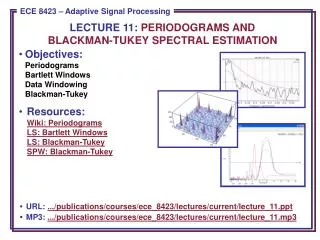
LECTURE 11: PERIODOGRAMS AND BLACKMAN-TUKEY SPECTRAL ESTIMATION. Objectives: Periodograms Bartlett Windows Data Windowing Blackman-Tukey Resources: Wiki: Periodograms LS: Bartlett Windows LS: Blackman- Tukey SPW: Blackman- Tukey.

Objectives: Periodograms Bartlett Windows Data Windowing Blackman-Tukey
E N D
Presentation Transcript
LECTURE 11: PERIODOGRAMS ANDBLACKMAN-TUKEY SPECTRAL ESTIMATION • Objectives:PeriodogramsBartlett WindowsData WindowingBlackman-Tukey • Resources:Wiki: PeriodogramsLS: Bartlett WindowsLS: Blackman-TukeySPW: Blackman-Tukey • URL: .../publications/courses/ece_8423/lectures/current/lecture_11.ppt • MP3: .../publications/courses/ece_8423/lectures/current/lecture_11.mp3
Introduction • Recall the power spectrum of a zero-mean stationary signal, x(n), with autocorrelation r(n), is defined by: • Our concern in this chapter is how to estimate the spectrum of x(n) from more than one finite set of data. For example, can we average successive estimates to obtain a better estimate than simply using all the data? (We considered a similar problem in the Pattern Recognition course.) • Methods of spectral analysis are divided into two groups: • Classical: operate as nonparameteric estimators and do not impose any model or structure on the data. • Modern: assume a model structure for the observed data and estimate the parameters of that model. • There are many possible ways to estimate the power spectrum derived from the autocorrelation function, such as: • Spectral estimates derived directly from the data are known as periodograms; those derived from the autocorrelation function are known as correlograms.
The Periodogram • The periodogram estimate of the power spectrum is defined as: • Of course, there are many ways to estimate the autocorrelation function. This particular estimate can be rewritten as: • This shows us the periodogram is the Fourier transform of the biased correlation estimate, r’(m). • Bias: r’(m) is itself biased with , but is also asymptotically unbiased because this estimate converges as M . • Variance: the periodogram is not a consistent estimator, which means increasing the number of data samples does not decrease the variance of the estimator at any one frequency. • Analytic evaluation of the variance is difficult, but we can demonstrate the problem both experimentally and analytically for a simple case.
Variance of the Periodogram – Experimental • Consider a simple AR process: • Generate 1024 samples: • Compute the periodogram for M=32, 128, 1024. • Observe that at any frequency the variance does not decrease, though the shape of the overall spectrum does change because the discrete frequencies used in the DFT are more closely spaced.
Variance of the Periodogram – Analytic • Consider the simple case when x(n) is a zero-mean IID Gaussian sequence. • The variance is given by: • The second term is easy to evaluate: • The first term is a bit more tedious, but, for a zero-mean IID process can be shown to reduce to: • The overall variance becomes: • However, observe that: • which means that our estimate of the autocorrelation is not consistent.
Generalizations • We can generalize our result by calculating the covariance of the periodogram for two frequencies: • For white input signals, the covariance between adjacent frequencies is zero (which is bad), but as M increases, the covariance remains zero, which means the variance does not decrease (refer to the plots on slide 3). • Similarly, for a signal generated by passing a zero-mean IID sequence through a linear time-invariant system, we can show: • The variance of the periodogram estimate is proportional to the square of the true spectrum. • Once again we observe the variance does not decay with increasing M, confirming that the periodogram is not a consistent estimator. • These observations led researchers to develop parametric techniques that were asymptotically consistent. These observations also led to ways to precondition the data so that the periodogram would be consistent or at the very least, more accurate.
The Bartlett Window • Recall our expression for the bias in the autocorrelation estimator: • We can view this as a windowing process: • This window is known as the triangular or Bartlett window. We recall that the impact on the spectrum is a convolution of the signal and the frequency response of the window:
The Modified Periodogram • For these reasons it is common to use a time-domain window with the periodogram: • We can show this is equivalent to: • Bias: • Variance and Consistency:
Averaging Periodograms • We can produce smooth estimates of the periodogram by averaging: • This is known as Bartlett’s estimate. • Bias: • Variance and Consistency: • This demonstrates that the variance decreases monotonically as the number of averages increases.
Blackman-Tukey Spectral Estimation • We can generalize the notion of windowing: • The window, wl(n), is a symmetric data window of length 2M1-1. • This estimate is known as the Blackman-Tukey or correlogram. When the window is rectangular, equivalent to the raw periodogram. • The window is symmetric so that the BT estimate is a real and even function. • As before, this can be viewed in the frequency domain as the convolution of the raw periodogram estimate and the frequency response of the window. • Bias: • Variance and Consistency: • Note that this is a consistent estimator because the variance tends to zero as M .
Summary • Introduced the periodogram. • Discussed the bias and variance of the raw periodogram. • We generalized this to a windowed periodogram and discussed the Bartlett window. • We also introduced the concept of a smoothed periodogram computed by averaging adjacent windows. • Finally, we introduced the Blackman-Tukey approach and discussed its bias and variance.