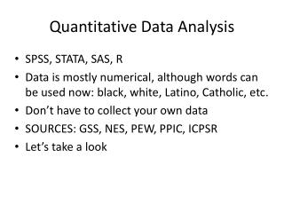
Quantitative Data Analysis

1. Quantitative Data Analysis JN602 Week 10 Veal Ch 13 & 14, SLT Chapter 11

2. Objectives • edit questionnaire and interview responses • set up the coding key for the data set and code the data • categorise data and create a data file • use SPSS, Excel or other software programs for data entry and data analysis • get a ‘feel’ for the data using univariate analysis • test the goodness of data • statistically test each hypothesis using bivariate analysis • interpret the computer results and prepare recommendations based on the quantitative data analysis

3. Quantitative Data Analysis Process • Data Preparation • Data Cleaning • Familiarisation – Frequencies, Means, Recoding • Data Analysis – Crosstabs, Statistics • Answering research questions • Graphics • Interpretation • Discussion and recommendations

4. Survey Analysis Overview

5. Data Preparation Getting Data Ready for Analysis • Editing data • Handling blank responses • Coding • Categorising • Entering data • Cleaning

6. Errors in the analysis process • Recording errors • Misreading of questionnaire • Multiple responses • Entry errors • Deliberate • Accidental: keying errors; misreading of responses

7. Entering data • Enter data from answer sheets directly into computer • Enter raw data through any software programme, eg SPSS Data Editor, Excel, text programme • Assign meaningful names to columns • Save regularly

8. Cleaning data • Possible code cleaning • Check that the distribution of the item is within the possible range of responses • If possible, computer program should not permit invalid entries • Contingency cleaning • Cleaning based on prior responses • E.g. males should not have responses regarding giving birth

9. Data entry:SPSS Variables specification • For each variable in the questionnaire, specify: • Name • Type – numeric or string • Width – max. no. of characters • Decimal places • Label – longer version of name • Values • Missing – blanks, no answer, etc. – see note • Columns – in Data View • Alignment – left, right, centre • Measure/data type – nominal, ordinal, scale – see note

10. A note on Measure/Data type • Nominal data = non-quantitative data: even if numerical codes are used, data cannot be added, multiplied etc. • Ordinal data = ranks: 1, 2, 3 etc. = first, second, third etc. • Scale data = fully numerical: can be added, multiplied, etc. • The type of data has implications for types of analysis which can be undertaken for individual variables

11. A note on ‘Missing’ values • If a no value response is entered for a variable (ie. = blank), SPSS treats this as a ‘Missing value’ • Not included in percentages etc. • You can specify other values as ‘Missing’ • eg. 0 could be specified as ‘No answer’ or ‘Not applicable’

12. Introduction to SPSS • SPSS uses two ‘windows’: • Variable View window • Data View window • User can ‘toggle’ between the two windows using the tabs at the bottom of the screen

13. SPSS Variable View window

14. SPSS Data View window

15. Completed ‘Variable View’ window

16. Types of research and approaches to analysis Starting an SPSS analysis session Analysis procedures Frequencies – one variable Frequencies – multiple variables Missing values Analysis procedures (continued): Checking for errors Multiple response Recode Means Attitude/Likert scales Crosstabulation Weighting Graphics Analysing Questionnaire Survey Data

17. Types of research and approaches to analysis

18. Starting an SPSS analysis session • Click on SPSS icon to start session OR select START, then PROGRAMS then SPSS • Select file from recently used files dialog box … or select MORE FILES and locate file, OR • Select FILE from menu bar, then OPEN, select FILES OF TYPE SPSS (.sav), then locate your file. • ‘Variable View’ and ‘Data View’ windows should appear.

19. The statistics approach • Concepts/terms/ideas used in statistics: • Forms of analysis • Measures of central tendency and dispersion • The idea of probabilistic statements • The normal distribution • Probabilistic statement formats • Significance • The null hypothesis • Dependent and independent variables

20. Forms of quantitative analysis • Univariate - simplest form,describe a case in terms of a single variable. • Bivariate - subgroup comparisons, describe a case in terms of two variables simultaneously. • Multivariate - analysis of two or more variables simultaneously.

21. Probabilistic statements It is only possible to estimate the probability that results obtained from a sample are true of the population – therefore statements on findings are probabilities.

22. Basis of probabilistic statements • Probability is based on the idea of drawing many random samples • Most results would be close to the population value • Some would be larger or smaller • A few would be very much larger or smaller • This distribution can be estimated using statistical theory • See Figure 14.1 – ‘bell-shaped’ Normal distribution

23. Fig. 14.1 Drawing repeated samples

24. Probabilistic statement formats • So far we have used 95% probability • this is sometimes expressed as 5% • and sometimes expressed as 0.05 • 99% probability is also used • also expressed 1% or 0.01 • 99.9% probability is occasionally used • Also expressed as 0.1% or 0.001 • Note particularly in correlation and ANOVA output

25. Significance • A finding which is unlikely to have happened by chance (ie. is ‘highly probable’) is described as ‘significant’ • Denoted by the probability of it occuring by chance (e.g. 0.05, 0.01, 0.001) • The larger the sample the greater the likelihood that a finding will be significant • But NB: small differences or weak relationships may not be socially or managerially significant – even when they are statistically significant

26. Univariate Analysis • Describing a case in terms of the distribution of attributes that comprise it. • Examples: course of study, sex, age Goals: • Provide reader with the fullest degree of detail regarding the data. • Present data in a manageable form.

27. Measures of central tendency and dispersion • Central tendency • The mean is the sum of scores in a distribution divided by the number of scores. • The mode is the most frequent score in a distribution. • The median is the mid-point or mid-score in a distribution • Dispersion • The range is: the highest score in a distribution minus the lowest score in the same distribution. • The variance is: the mean of the squared deviation scores about the mean of a distribution. • The standard deviation is: the square root of the variance

28. Descriptive statistics

29. Frequency tables • For presentation of CATEGORICAL data • Nominal or ordinal responses • Eg. Day of week, sex • Present the distribution of a small number of categories

30. Day of week

31. Chart of frequencies

32. Bivariate Analysis • Describe a case in terms of two variables simultaneously. • Aim is to test the relationship between the independent (explanatory) variable and the dependent variable • Example: • Gender • Amount of exercise

33. Fig. 14.2 Dependent & independent variables Does this look familiar?

34. Null hypothesis • Setting up two mutually incompatible hypotheses: • if one is true the other must be false • The ‘null’ hypothesis and the alternative hypothesis • H0 = Null hypothesis: there is no difference/relationship • H1 = Alternative hypothesis: there is a difference/relationship

35. Fig. 14.3a: What tests?

36. Fig. 14.3b : What tests?

37. Data file • To demonstrate SPSS statistical procedures: • Data from student background survey • Data from online diary survey • PDA survey data available next week

38. Chi-square • Testing the relationship between two variables presented in a frequency crosstabulation. • Null/alternative hypotheses: • H0 - there is no relationship between exercise activity and gender in the population • H1 - there is a relationship between exercise activity and gender in the population. • SPSS - procedures p. 260 - Figure 14.4

39. Fig. 14.6 Chi-square – distribution

40. Interpreting Chi-square output - 1 • Degrees of freedom • (Number of rows -1) x (Number of columns -1) • Expected counts rule: • Expected count = cell frequency if there was no relationship at all between the variables • Should be: no more than one fifth of cells with expected counts of less than 5 • Should be: no cells with expected count of less than 1 • If rule is violated: try combining rows or columns • Presentation of Chi-square results – See Fig. 14.7

41. Interpreting Chi-square output - 2 • Value of chi-square: • If value is in the 5% zone (ie. Probability is less that .05) it is an unlikely value and Null Hypothesis is rejected. • Value is 6.588 and probability is 0.037 or 3.7%, so Null Hypothesis is rejected • there is a significant difference in enrolment pattern between men and women. • Presentation of Chi-square results – See Fig. 14.7

42. Chi-squared output

43. Comparing two means: t-test • Situation 1: two variables applying to all members of the sample • Eg. Compare time spent on exercise and time spent on study • Paired samples t-test • Situation 2: sample is divided in two • Eg. Compare average happiness levels in different activities • Independent samples t-test

44. Compare two means: t-test – t distribution

45. Compare 2 means: Independent samples t-test

46. Compare 2 means: Independent samples t-test • Reading t-tests • Example 1: Enjoyment and happiness by activity • Happiness: in class mean 2.53, at work 2.73 • H0 Null hypothesis: there is no difference between these two • t value = -0.712; Probability = 0.478 (which is > 0.05) • Accept the null hypothesis – there is no significant difference

47. Compare 3+ means: One-way Analysis of Variance (ANOVA) • Comparing a range of means – see Fig. 14.11 • SPSS – see procedure pp. 243-44 • H0 Null hypothesis: each of the group means is equal to the overall mean • H1 Alternative hypothesis: there is a difference between group means

48. One-way Analysis of Variance (ANOVA)

49. One-way Analysis of Variance (ANOVA): the idea of Variance

50. One-way Analysis of Variance (ANOVA) • SPSS - procedure p. 271 – see Fig. 14.13