Quantitative Data Analysis
Quantitative Data Analysis. Edouard Manet: In the Conservatory, 1879. Quantification of Data Introduction To conduct quantitative analysis, responses to open-ended questions in survey research and the raw data collected using qualitative methods must be coded numerically.


Quantitative Data Analysis
E N D
Presentation Transcript
Quantitative Data Analysis Edouard Manet: In the Conservatory, 1879
Quantification of Data • Introduction • To conduct quantitative analysis, responses to open-ended questions in survey research and the raw data collected using qualitative methods must be coded numerically.
Quantification of Data • Introduction (Continued) • Most responses to survey research questions already are recorded in numerical format. • In mailed and face-to-face surveys, responses are keypunched into a data file. • In telephone and internet surveys, responses are automatically recorded in numerical format.
Quantification of Data • Developing Code Categories • Coding qualitative data can use an existing scheme or one developed by examining the data. • Coding qualitative data into numerical categories sometimes can be a straightforward process. • Coding occupation, for example, can rely upon numerical categories defined by the Bureau of the Census.
Quantification of Data • Developing Code Categories (Continued) • Coding most forms of qualitative data, however, requires much effort. • This coding typically requires using an iterative procedure of trial and error. • Consider, for example, coding responses to the question, “What is the biggest problem in attending college today.” • The researcher must develop a set of codes that are: • exhaustive of the full range of responses. • mutually exclusive (mostly) of one another.
Quantification of Data • Developing Code Categories (Continued) • In coding responses to the question, “What is the biggest problem in attending college today,” the researcher might begin, for example, with a list of 5 categories, then realize that 8 would be better, then realize that it would be better to combine categories 1 and 5 into a single category and use a total of 7 categories. • Each time the researcher makes a change in the coding scheme, it is necessary to restart the coding process to code all responses using the same scheme.
Quantification of Data • Developing Code Categories (Continued) • Suppose one wanted to code more complex qualitative data (e.g., videotape of an interaction between husband and wife) into numerical categories. • How does one code the many statements, facial expressions, and body language inherent in such an interaction? • One can realize from this example that coding schemes can become highly complex.
Quantification of Data • Developing Code Categories (Continued) • Complex coding schemes can take many attempts to develop. • Once developed, they undergo continuing evaluation. • Major revisions, however, are unlikely. • Rather, new coders are required to learn the existing coding scheme and undergo continuing evaluation for their ability to correctly apply the scheme.
Quantification of Data • Codebook Construction • The end product of developing a coding scheme is the codebook. • This document describes in detail the procedures for transforming qualitative data into numerical responses. • The codebook should include notes that describe the process used to create codes, detailed descriptions of codes, and guidelines to use when uncertainty exists about how to code responses.
Quantification of Data • Data Entry • Data recorded in numerical format can be entered by keypunching or the use of sophisticated optical scanners. • Typically, responses to internet and telephone surveys are entered directly into a numerical data base. • Cleaning Data • Logical errors in responses must be reconciled. • Errors of entry must be corrected.
Quantification of Data • Collapsing Response Categories • Sometimes the researcher might want to analyze a variable by using fewer response categories than were used to measure it. • In these instances, the researcher might want to “collapse” one or more categories into a single category. • The researcher might want to collapse categories to simplify the presentation of the results or because few observations exist within some categories.
Quantification of Data • Collapsing Response Categories: Example • ResponseFrequency • Strongly disagree 2 • Disagree 22 • Neither agree nor disagree 45 • Agree 31 • Strongly Agree 1
Quantification of Data • Collapsing Response Categories: Example • One might want to collapse the extreme responses and work with just three categories: • ResponseFrequency • Disagree 24 • Neither agree nor disagree 45 • Agree 32
Quantification of Data • Handling “Don’t Knows” • When asking about knowledge of factual information (“Does your teenager drink alcohol?”) or opinions on a topic the subject might not know much about (“Do school officials do enough to discourage teenagers from drinking alcohol?”), it is wise to include a “don’t know” category as a possible response. • Analyzing “don’t know” responses, however, can be a difficult task.
Quantification of Data • Handling “Don’t Knows” (Continued) • The research-on-research literature regarding this issue is complex and without clear-cut guidelines for decision-making. • The decisions about whether to use “don’t know” response categories and how to code and analyze them tends to be idiosyncratic to the research and the researcher.
Quantitative Data Analysis • Descriptive statistics attempt to explain or predict the values of a dependent variable given certain values of one or more independent variables. • Inferential statistics attempt to generalize the results of descriptive statistics to a larger population of interest.
Quantitative Data Analysis • Data Reduction • The first step in quantitative data analysis is to calculate descriptive statistics about variables. • The researcher calculates statistics such as the mean, median, mode, range, and standard deviation. • Also, the researcher might choose to collapse response categories for variables.
Quantitative Data Analysis • Measures of Association • Next, the researcher calculates measures of association: statistics that indicate the strength of a relationship between two variables. • Measures of association rely upon the basic principle of proportionate reduction in error (PRE).
Quantitative Data Analysis • Measures of Association (Continued) • PRE represents how much better one would be at guessing the outcome of a dependent variable by knowing a value of an independent variable. • For example: How much better could I predict someone’s income if I knew how many years of formal education they have completed? If the answer to this question is “37% better,” then the PRE is 37%.
Quantitative Data Analysis • Measures of Association (Continued) • Statistics are designated by Greek letters. • Different statistics are used to indicate the strength of association between variables measured at different levels of data. • Strength of association for nominal-level variables is indicated by λ (lambda). • Strength of association for ordinal-level variables is indicated by γ (gamma). • Strength of association for interval-level variables is indicated by correlation (r).
Quantitative Data Analysis • Measures of Association (Continued) • Covariance is the extent to which two variables “change with respect to one another.” • As one variable increases, the other variable either increases (positive covariance) or decreases (negative covariance). • Correlation is a standardized measure of covariance. • Correlation ranges from -1 to +1, with figures closer to one indicating a stronger relationship.
Quantitative Data Analysis • Measures of Association (Continued) • Technically, covariance is the extent to which two variables co-vary about their means. • If a person’s years of formal education is above the mean of education for all persons and his/her income is above the mean of income for all persons, then this data point would indicate positive covariance between education and income.
Statistics • Introduction • To make inferences from descriptive statistics, one has to know the reliability of these statistics. • In the same sense that the distribution of one variable has a standard deviation, a parameter estimate has a standard error—the distribution of the estimate from its mean with respect to the normal curve.
Statistics • Introduction (Continued) • To better understand the concepts standard deviation and standard error, and why these concepts are important to our course, please review the presentation regarding standard error. • Presentation on Standard Error.
Statistics • Types of Analysis • The presentation on inferential statistics will cover univariate, bivariate and multivariate analysis. • Univariate Analysis: • Mean. • Median. • Mode. • Standard deviation.
Statistics • Types of Analysis (Continued) • Bivariate Analysis • Tests of statistical significance. • Chi-square. • Multivariate Analysis: • Ordinary least squares (OLS) regression. • Path analysis. • Time-series analysis. • Factor analysis. • Analysis of variance (ANOVA).
Univariate Analysis • Distributions • Data analysis begins by examining distributions. • One might begin, for example, by examining the distribution of responses to a question about formal education, where responses are recorded within six categories. • A frequency distribution will show the number and percent of responses in each category of a variable.
Univariate Analysis • Central Tendency • A common measure of central tendency is the average, or mean, of the responses. • The median is the value of the “middle” case when all responses are rank-ordered. • The mode is the most common response. • When data are highly skewed, meaning heavily balanced toward one end of the distribution, the median or mode might better represent the “most common” or “centered” response.
Univariate Analysis • Central Tendency (Continued) • Consider this distribution of respondent ages: • 18, 19, 19, 19, 20, 20, 21, 22, 85 • The mean equals 27. But this number does not adequately represent the “common” respondent because the one person who is 85 skews the distribution toward the high end. • The median equals 20. • This measure of central tendency gives a more accurate portrayal of the “middle of the distribution.”
Univariate Analysis • Dispersion • Dispersion refers to the way the values are distributed around some central value, typically the mean. • The range is the distance separating the lowest and highest values (e.g., the range of the ages listed previously equals 18-85). • The standard deviation is an index of the amount of variability in a set of data.
Univariate Analysis • Dispersion (Continued) • The standard deviation represents dispersion with respect to the normal (bell-shaped) curve. • Assuming a set of numbers is normally distributed, then each standard deviation equals a certain distance from the mean. • Each standard deviation (+1, +2, etc.) is the same distance from each other on the bell-shaped curve, but represents a declining percentage of responses because of the shape of the curve (see: Chapter 7).
Univariate Analysis • Dispersion (Continued) • For example, the first standard deviation accounts for 34.1% of the values below and above the mean. • The figure 34.1% is derived from probability theory and the shape of the curve. • Thus, approximately 68% of all responses fall within one standard deviation of the mean. • The second standard deviation accounts for the next 13.6% of the responses from the mean (27.2% of all responses), and so on.
Univariate Analysis • Dispersion (Continued) • If the responses are distributed approximately normal and the range of responses is low—meaning that most responses fall close to the mean—then the standard deviation will be small. • The standard deviation of professional golfer’s scores on a golf course will be low. • The standard deviation of amateur golfer’s scores on a golf course will be high.
Univariate Analysis • Continuous and Discrete Variables • Continuous variables have responses that form a steady progression (e.g., age, income). • Discrete (i.e., categorical) variables have responses that are considered to be separate from one another (i.e., sex of respondent, religious affiliation).
Univariate Analysis • Continuous and Discrete Variables • Sometimes, it is a matter of debate within the community of scholars about whether a measured variable is continuous or discrete. • This issue is important because the statistical procedures appropriate for continuous-level data are more powerful, easier to use, and easier to interpret than those for discrete-level data, especially as related to the measurement of the dependent variable.
Univariate Analysis • Continuous and Discrete Variables (Continued) • Example: Suppose one measures amount of formal education within five categories: less than hs, hs, 2-years vocational/college, college, post-college). • Is this measure continuous (i.e., 1-5) or discrete? • In practice, five categories seems to be a cutoff point for considering a variable as continuous. • Using a seven-point response scale will give the researcher a greater chance of deeming a variable to be continuous.
Bivariate Analysis • Introduction • Bivariate analysis refers to an examination of the relationship between two variables. • We might ask these questions about the relationship between two variables: • Do they seem to vary in relation to one another? That is, as one variable increases in size does the other variable increase or decrease in size? • What is the strength of the relationship between the variables?
Bivariate Analysis • Introduction (Continued) • Divide the cases into groups according to the attributes of the independent variable (e.g., men and women). • Describe each subgroup in terms of attributes of the dependent variable (e.g., what percent of men approve of sexual equality and what percent of women approve of sexual equality).
Bivariate Analysis • Introduction (Continued) • Read the table by comparing the independent variable subgroups with one another in terms of a given attribute of the dependent variable (e.g., compare the percentages of men and women who approve of sexual equality). • Bivariate analysis gives an indication of how the dependent variable differs across levels or categories of an independent variable. • This relationship does not necessarily indicate causality.
Bivariate Analysis • Introduction (Continued) • Tables that compare responses to a dependent variable across levels/categories of an independent variable are called contingency tables (or sometimes, “crosstabs”). • When writing a research report, it is common practice, even when conducting highly sophisticated statistical analysis, to present contingency tables also to give readers a sense of the distributions and bivariate relationships among variables.
Bivariate Analysis • Tests of Statistical Significance • If one assumes a normal distribution, then one can examine parameters and their standard errors with respect to the normal curve to evaluate whether an observed parameter differs from zero by some set margin of error. • Assume that the researcher sets the probability of a Type-1 error (i.e., the probability of assuming causality when there is none) at 5%. • That is, we set our margin of error very low, just 5%.
Bivariate Analysis • Tests of Statistical Significance (Continued) • To evaluate statistical significance, the researcher compares a parameter estimate to a “zero point” on a normal curve (its center). • The question becomes: Is this parameter estimate sufficiently large, given its standard error, that, within a 5% probability of error, we can state that it is not equal to zero?
Bivariate Analysis • Tests of Statistical Significance (Continued) • To achieve a probability of error of 5%, the parameter estimate must be almost two (i.e., 1.96) standard deviations from zero, given its standard error. • Sometimes in sociological research, scholars say “two standard deviations” in referring to a 5% error rate. Most of the time, they are more precise and state 1.96.
Bivariate Analysis • Tests of Statistical Significance (Continued) • Consider this example: • Suppose the unstandardized estimate of the effect of self-esteem on marital satisfaction equals 3.50 (i.e., each additional amount of self-esteem on its scale results in 3.50 additional amount of marital satisfaction on its scale). • Suppose the standard error of this estimate equals 1.20.
Bivariate Analysis • Tests of Statistical Significance (Continued) • If we divide 3.50 by 1.20 we obtain the ratio of 2.92. This figure is called a t-ratio (or, t-value). • The figure 2.92 means that the estimate 3.50 is 2.92 standard deviations from zero. • Based upon our set margin of error of 5% (which is equivalent to 1.96 standard deviations), we can state that at prob. < .05, the effect of self-esteem on marital satisfaction is statistically significant.
Bivariate Analysis • Tests of Statistical Significance (Continued) • The t-ratio is the ratio of a parameter estimate to its standard error. • The t-ratio equals the number of standard deviations that an estimate lies from the “zero point” (i.e., center) of the normal curve.
Bivariate Analysis • Tests of Statistical Significance (Continued) • Why do we state that we need to have 1.96 standard deviations from the zero point of the normal curve? • Recall the area beneath the normal curve: • The first standard deviation covers 34.1% of the observations on one side of the zero point. • The second standard deviation covers the next 13.6% of the observations.
Bivariate Analysis • Tests of Statistical Significance (Continued) • Let’s assume for a moment that our estimate is greater than the “real” effect of self-esteem on marital satisfaction. • Then, at 1.96 standard deviations, we have covered the 50% probability below the “real” effect, and we have covered 34.1% + 13.4% probability above this effect. • In total, we have accounted for 97.5% of the probability that our estimate does not equal zero.
Bivariate Analysis • Tests of Statistical Significance (Continued) • That leaves 2.5% of the probability above the “real” estimate. • But we have to recognize that our estimate might have fallen below the “real” estimate. • So, we have the probability of error on both sides of “reality.” • 2.5% + 2.5% equals 5% • This is our set margin of error!
Bivariate Analysis • Tests of Statistical Significance (Continued) • Thus, inferential statistics are calculated with respect to the properties of the normal curve. • There are other types of distributions besides the normal curve, but the normal distribution is the one most often used in sociological analysis.