Quantitative Data Analysis
Quantitative Data Analysis. Quantitative data Analysis. Numerical representation and manipulation of observations for the purpose of describing and explaining the phenomena that those observations reflect.

Quantitative Data Analysis
E N D
Presentation Transcript
Quantitative data Analysis • Numerical representation and manipulation of observations for the purpose of describing and explaining the phenomena that those observations reflect. • In economics field also known as econometrics. It concerns the development of statistical methods to test the validity of economic theories.
The knowledge of econometrics is crucial in conducting the data analysis in economics research. • Basic knowledge of econometric theory is necessary to understand what may (or may not) be done in applied quantitative economic research, when we deal with secondary data.
Goals, objectives and aims of Econometrics • Formulation of econometric models in an empirically testable form. • Empirical verification (Estimation and testing) of these models with observed data [estimating coefficients of economic relationships]. • Making prediction, forecasting future values of economic variables or phenomena and policy recommendation
Procedure of quantitative data analysis • Data entry – enter the data into the package or Excel spreadsheet. • Various econometrics software such as EViews (Econometrics Views), SHAZAM, RATS, MICROFIT, PcGive, PcFilm, TSP, GAUSS). It is part of the process of data collection before the estimation process. • Primary data analysis package such as SPSS.
After the data entry to the relevant program (example: E-views) we are ready for the estimation or the data. • To check on the data, we may plot the data to ensure it is free from human error. • Despite that now days, the data are ready in excel format in most of the central banks, IFS or some other institutions.
The estimation (statistical) techniques could includes descriptive, regression (simple and multivariate) and forecasting analysis. • Hypothesis testing is usually adopted here. • Diagnostic checking for the model
Interpretation of the results based on economic theories. Please be advice that the interpretation is not limited to the statistical interpretation (example: significant or not). • Make conclusion, implication, policies and to resemble the reality of the world. • Present or send for publication consideration the term paper of economics research.
Descriptive Analysis • Descriptive statistics fall into one of two categories: measures of central tendency (mean, median, and mode) or measures of dispersion (standard deviation and variance).
Measures of central tendency • mean • sum all values in distribution, then divide by total number of values • median • middle point within entire range of values • not distorted by outliers • mode • most frequently occurring value
Measures of dispersion • amount of variation in a sample • compare levels of variation in different samples • is there more variability in a variable in sample x than in sample y? • standard deviation • average amount of variation around the mean • impact of outliers is reduced
Regression Analysis • Regression is the most commonly used tool in econometric analysis. • Study of relationship between one variable called the explained/dependent variable and one or more other variables called independent/explanatory variable(s). • y - explained/dependent variable • x - independent/explanatory variable
Aims of Regression • To examine whether there exists a significant relationship between any of the x’s and y. • To analyze the effects of changing one or more of the x’s on y. • To forecast the value of y for a given set of x’s.
Bivariate analysis(analysis of two variables) • explores relationships between variables • search for co-variance and correlations • cannot establish causality • can sometimes infer the direction of a causal relationship • if one variable preceded the other
Multivariate analysis(three or more variables) • the relationship between two variables might be spurious • each variable could be related to a separate, third variable
Deterministic and Stochastic Relationships • There are two types of relationships: • deterministic or exact relationships. • Take the following model: • y = 3500 + 100x • The values for y can be exactly determined for given values of x. • stochastic or statistical relationships which do not give unique values of y for given values of x. • Suppose the model is specified as: • y = 3500 + 100x + u • By defining y in probabilistic terms, it cannot be exactly determined for given values of x. • Statistical relations are specified in probabilistic terms. • Regression uses statistical models.
Simple Vs Multiple Regression • Simple Regression - one independent variable • Multiple Regression - more than one independent variable
Why add an error term? • The relationship between economic variables is unlikely to be exact because of stochastic error. • Stochastic error is also known as random error, disturbance, or simply error term. • A (random) disturbance or error must be included in the exact relationships postulated by economic theory and mathematical economics in order to make them stochastic (in order to reflect the fact that in the real world, economic relationships among economic variables are inexact and somewhat erratic).
To account for the inexact relationship between economic variables, an error term must be included in our regression equation. • where stands for the error term. • Equation above is made up of deterministic component ( ) and stochastic component ( ). • The deterministic component determines the expected value of Y. This component tells us exactly by how much a change in X will be reflected in the change in Y.
However, in the real world, it is unlikely that variation in Y is solely explained by variation in X. • There are some variations in Y that cannot be explained by the model. • Econometric admit the existence of such unexplained variation by explicitly including a stochastic component in the model. • The inclusion of a (random) disturbance or error term (with well-defined probabilistic properties) is required in regression analysis for three important reasons.
Since the purpose of theory is to generalize and simplify, economic relationships usually include only the most important forces at work. This means that numerous other variables with slight and irregular effects are not included. The error term can be viewed as representing the net effect of this large number of small and irregular forces at work.
The inclusion of the error term can be justifies in order to take into consideration the net effect of possible errors in measuring the dependent variable or variable being explained. • Since human behavior usually differs in a random way under identical circumstances the disturbance or error term can be used to capture this inherently random human behavior. This error term thus allow for individual random deviations from the exact and deterministic relationships postulated by economic theory and mathematical economics.
Ordinary Least Squares (OLS) Method • The most common form of regression, however, is linear regression, and the least squares method to find an equation that best fits a line representing what is called the regression of y on x. • One is interested in finding the perfect line, such that there is one and only one line (represented by equation) that perfectly represents, or fits the data, regardless of how scattered the data points.
The slope of the line (equation) provides information about predicted estimated coefficients (or beta weights) for x and y (independent and dependent variables). • As it gives the best straight line that fits the sample of XY observations, it minimizes the sum of squared (vertical) deviations of each observed point on the graph from the straight line. Ordinary Least Square is to minimize Residual Sum of Squares (RSS).
Example: OLS • minimize Residual Sum of Squares (RSS) Evan Lau (CHAP 10)
Correlation (r) • Correlation coefficient used to a measure the strength and direction of the relationship between two variables. • Interpretation of a correlation coefficient does not even allow the slightest hint of causality. The most a researcher can say is that the variables share something in common; that is, are related in some way. • The more two things have something in common, the more strongly they are related. There can also be negative relations
0.8 to 1.0 very strong 0.6 to 0.8 strong 0.4 to 0.6 moderate 0.2 to 0.4 weak 0 to 0.2 very weak • The following table lists the interpretations for various correlation coefficients. It is same applied to negative correlation
Coefficient of Determination, R2 • TSS = ESS + RSS TSS = the total sum of square of Y ESS = explained sum of squares RSS = the residual sum of square = i2
Coefficient of Determination, R2 • Percentage of the total variation in dependent variable is explained by all the independent variables. • R2 reflects the “goodness of fit” of the estimated regression model. For example, if R2=0.89, 89% of variation in Y is explained by all the X’s. • The higher the R2, the better the estimated regression model fits the sample data.
As number of independent variables increase (for example from 2 independents variables increase to 4), R2 will also increase. Thus, it is not suitable for comparing two regression models with the same dependent variable but difference number of independent variables. • This is because R2 does not take into consideration of degree of freedom. To mitigate this problem, we can used , the adjusted R2 (adjusted for degrees of freedom)
Diagnostic Checking • Several diagnostic checking upon the completion of Econometrics course • Autocorrelation - Durbin-Watson d Test, Durbin-Watson h Test and Breusch-Godfrey (BG) LM Test. • Heteroscedasticity - Goldfeld-Quant test, Breusch-Pagan-Godfrey test and White test • Multicollinearity (no particular formal testing procedure) • Stability test - Chow test, CUSUM (cumulative sum) and CUSUM square) • Normality (Jarque-Bera Test) • ARCH (autoregressive conditional heteroscedasticity) • Specification test - Ramsey's RESET (regression specification error) test
A sound modelling strategy • General to Specific (Hendry’s approach) • start with all the variables and all full sample • reduce and refine as necessary • In choosing such a model, we will have to try several specifications before we finally settle down on the final model. • That is why Hendry approach is also known as TTT methodology that is Test, test and test.
Steps in Hendry approach (i) Theory (ii) Anticipated Regression Model (iii) Data Collection (iv) General Model (v) Diagnostic Checks and Refinement (vi) Specific Model (vii) Revise Theory? (iix) Present Final Model (the specific model)