EROS (Crave & Davy, 2001)

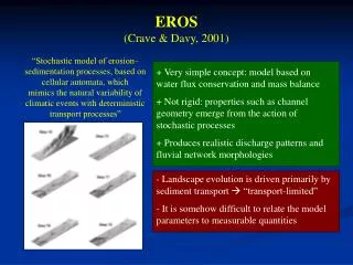
EROS (Crave & Davy, 2001) “Stochastic model of erosion–sedimentation processes, based on cellular automata, which mimics the natural variability of climatic events with deterministic transport processes” + Very simple concept: model based on water flux conservation and mass balance + Not rigid: properties such as channel geometry emerge from the action of stochastic processes + Produces realistic discharge patterns and fluvial network morphologies - Landscape evolution is driven primarily by sediment transport  “transport-limited” - It is somehow difficult to relate the model parameters to measurable quantities

CHILD (Tucker at al., 2001) + User friendly + Includes a wide range of fluvial incision laws and tectonic scenarios + Uses a Triangulated Irregular Network + Stochastic rainfall variability - No landsliding algorithm - Some properties are relatively rigid, e.g. channel geometry defined by hydraulic scaling relationships

CHILD (Tucker at al., 2001) Uplift rate increased 1 Ma ago Example 1: landscape response to tectonic perturbation; application to the Central Apennines, Italy (Attal et al., 2008)

CHILD (Tucker at al., 2001) Example 1: landscape response to tectonic perturbation; application to the Central Apennines, Italy (Attal et al., 2008)

Profile shape and landscape morphology Example 1: landscape response to tectonic perturbation; application to the Central Apennines, Italy (Attal et al., 2008) Fiamignano Fault Time = 0.0 My Questions: can we reproduce the catchments’ morphology using a simple detachment-limited fluvial erosion law (model testing)? What is the effect of “dynamic channel adjustment” (sensitivity analysis)? Fault Uplift

Profile shape and landscape morphology Example 1: landscape response to tectonic perturbation; application to the Central Apennines, Italy (Attal et al., 2008) Time = 0.2 My

Profile shape and landscape morphology Basin internally drained Example 1: landscape response to tectonic perturbation; application to the Central Apennines, Italy (Attal et al., 2008) Time = 1.6 My Slope < 0

Profile shape and landscape morphology Basin internally drained Example 1: landscape response to tectonic perturbation; application to the Central Apennines, Italy (Attal et al., 2008) Time = 2.2 My • Simple DL model makes relatively good predictions. • Role of CHANNEL NARROWING (morphology + response time) Slope < 0

CHILD (Tucker at al., 2001) No vegetation Example 2 (sensitivity analysis): effect of vegetation and wildfires on landscape development; application to the Oregon Coast Range (Istanbulluoglu & Bras, 2005)  Vegetation cover and changes in cover through time (landslides, wild fires) strongly affects landscape morphology (relief, drainage density) Static vegetation cover (Roering et al., 1999)

Modelling landscape evolution Where are we? Models are getting more and more complex, include more and more processes and parameters, but… Some essential key issues need to be addressed:  Role of sediment (fluvial erosion),  Role of “life” (vegetation, bioturbation, etc.),  Role of climate

http://coastalchange.ucsd.edu/ Climate and landscape evolution  Climate is highly variable at geological time scales  Climate (e.g. temperature, rainfall, storminess) strongly influences erosion rates and processes Hillslopes: landsliding, freeze-thaw cycles Rivers: erosion occurs during discrete events = floods which mobilize sediments

http://www.cru.uea.ac.uk/cru/info/ Climatic Research Unit, UEA Norwich Climate and landscape evolution Problem: most studies involving landscape evolution modelling assume that climate parameters are constant over millions of years! Solution: coupling landscape evolution models with climate models Problem: SCALE!!! LANDSCAPE EVO. MODELS TIME STEP = 10s hours to 1000s year GRID RESOLUTION = 10s to 1000s meters CLIMATE MODELS TIME STEP = 15 minutes to a few hours MIN GRID RESOLUTION = 100 km!

Vision for the future? The aim: • Solving the scale problems to couple climate and landscape development models • realistic predictions of landscape evolution as a result of climate variability + feedbacks between topography and climate • predictions at varied time and space scales (from minutes to millions of years, from a small stream to whole countries!) http://www.cru.uea.ac.uk/cru/info/ Climatic Research Unit, UEA Norwich

Tectonics The Channel-Hillslope Integrated Landscape Development (CHILD) model (Tucker et al., 2001) PAUSE Climate parameters Hillslope transport + landslide threshold Initial topography Fluvial sediment transport + deposition + bedrock erosion Additional parameters and algorithms: fluvial hydraulic geometry, bedrock and sediment characteristics, role of vegetation, etc. CHILD

The Channel-Hillslope Integrated Landscape Development (CHILD) model (Tucker et al., 2001)

The Channel-Hillslope Integrated Landscape Development (CHILD) model (Tucker et al., 2001) If OPTDETACHLIM = 1  E = KAmSn

The Channel-Hillslope Integrated Landscape Development (CHILD) model (Tucker et al., 2001) To set in the .in file τ = ktqmbSnb = kt(Q/W)mbSnb Calculated by CHILD We will consider: Erosion  Specific Stream power (Law 2): E  Ω/ W E = K Q S / W  mb = 0.6; nb = 0.7; pb = 1.5; τc = 0 To set in the .in file E = kb (τ – τc)pb kt = 1197 (typical value for bedrock rivers) kb or kr = poorly constrained parameters

The Channel-Hillslope Integrated Landscape Development (CHILD) model (Tucker et al., 2001) CHILD user guide

The Channel-Hillslope Integrated Landscape Development (CHILD) model (Tucker et al., 2001) Channel Width is calculated at each time step for every node: W = kwQωsQb(ωb-ωs) = kwQωs if ωs = ωb

Visualizing the output using Matlab ctrisurf(‘filename’, ts, 0)

EROS (Crave & Davy, 2001)