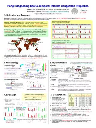
Pong: Diagnosing Spatio-Temporal Internet Congestion Properties
10 likes | 146 Vues
5. 6. 7. 3. 4. 9. 10. 11. 8. 2. 1. 9. 3. 8. 12. 4. 10. 11. 5. 7. 6. 1. 2. 5. 6. 7. 3. 4. 9. 10. 11. 8. 0.53s on/off. 2. 1. 0.37s on/off. 0.71s on/off. 9. 3. 8. 12. 4. 10. 11. 5. 7. 6. 1. 2. 0.47s on/off. 0.83s on/off. 0.53s on/off. 0.37s on/off.

Pong: Diagnosing Spatio-Temporal Internet Congestion Properties
E N D
Presentation Transcript
5 6 7 3 4 9 10 11 8 2 1 9 3 8 12 4 10 11 5 7 6 1 2 5 6 7 3 4 9 10 11 8 0.53s on/off 2 1 0.37s on/off 0.71s on/off 9 3 8 12 4 10 11 5 7 6 1 2 0.47s on/off 0.83s on/off 0.53s on/off 0.37s on/off 0.71s on/off 0.29s on/off 0.63s on/off Link 7 Demote Promote 1 1 Congestion points located by Pong Graph: Congestion count vs. link # Recent 10 seconds (updated every 10 seconds) Recent 30 seconds (updated every 10 seconds) Recent 1 minute (updated every 10 seconds) 1.6 4.8 10.4 0.8 2.4 5.2 1 2 3 4 5 6 7 8 9 1 2 3 4 5 6 7 8 9 1 2 3 4 5 6 7 8 9 Recent 3 minutes (updated every 1 minute) Recent 10 minutes (updated every 1 minute) Recent 30 minutes (updated every 10 minutes) 35.2 112.7 242.2 17.6 56.4 121.1 2 3 4 9 5 8 7 6 9 1 2 3 4 5 6 7 8 9 1 2 3 4 5 6 7 8 9 1 2 3 4 5 6 7 8 9 Recent 1 hour (updated every 10 minutes) Recent 3 hours (updated every 1 hour) Recent 6 hours (updated every 1 hour) 473.4 581.9 581.9 236.7 290.9 290.9 1 2 3 4 5 6 7 8 9 1 2 3 4 5 6 7 8 9 1 2 3 4 5 6 7 8 9 Congestion status traced by Pong Graph: Congestion intensity vs. time Receiver Sender probe Link 1 Link 2 Link 3 probe Congestion Link 4 Link 5 Link 6 Link # ~ Link 7 Link 8 Link 9 f Pairing Congestion s Internet Probe d Pair up an s probe with a d probe f Control channel b Complementary d probe s pong_rcv pong_snd D D S S d Control Control b File File pong_daemon pong_daemon A Symmetric Path Scenario Web front end f f Pairing s s S S D D Collect data Control & monitor Web front end pong File Statistic kits b d Complementary d probe Observed by b probe only pongc b No complementary d probe available Use f, s, d probe only Use, f, s, b probe only Two Minor Scenarios Probe Probe D S Update Congestion Count Detect Switch Point Probe Probe Probe Probe Probe S D Congestion Count > Threshold Correlate probes to neighboring nodes Congestion Point Detected Reuse probes to all intermediate nodes Switch Point Approach • Simulation-based Evaluation using ns2 • Emulation Experiments on Emulab Testbed • Self-consistency Validation through Large-scale Internet Experiments Pong: Diagnosing Spatio-Temporal Internet Congestion Properties Leiwen Deng and Aleksandar Kuzmanovic, Northwestern University Northwestern Networks Group (http://networks.cs.northwestern.edu) Supported by Cisco Collaborative Research 1. Motivation and Approach Motivation. The ability to accurately detect congestion events in the Internet and reveal their spatial (where they happen) and temporal (how long they last) properties would significantly improve our understanding of how the Internet operates. Locating congestion points. Pong is a tool that detects congestion on a unidirectional path with high resolution and high accuracy. It locates congestion on granularity of a single link. It performs well in detecting multiple congested links on the forward path and in decoupling congested links on the backward path. Monitoring congestion points. Once a congested link is detected, Pong traces congestion status on that link. The light-weight nature of Pong makes Pong also a competent network monitoring tool rather than only an on-demand probing tool. The web front end and command line interface (CLI) provided by Pong facilitate measurement and monitoring jobs. An example scenario: There is congestion on link 1, 5 and 8. We probe the path from the sender and the receiver with Pong. We quantify congestion properties on each link with two measures – congestion count and congestion intensity. 2. Methodology 3. Implementation Source code and sample measurement outputs of Pong are available at http://networks.cs.northwestern.edu/pong • Highlights • Tested on Fedora Core 4/5 Linux. • Use libpcap to retrieve kernel level timestamps. • Single path measurement or monitoring; large-scale Internet measurement. • Extensive log information for error diagnosing. • Coordinated Probing General Scenario Four probing packets in a coordinated way: • Components Illustration of Pong • Locating Congestion Points • Tracing Congestion Status Tracing Congestion Status of Detected Congestion Points 5. Measurement 4. Evaluation Congestion Measure Spatial Taxonomy • Experimental Setup • A large-scale Internet experiment using 334 PlanetLab hosts (167 senders and 167 receivers). • Measured 21,861 paths within 10 days. • Measure each path for 100 minutes. An Emulab Experiment Example • 12 nodes, 11 links (100Mbps, 2ms). • Use TCP on/off traffic to build congestion on links. • Measurement Results • The network edge is 4.5 times more congested than the core on average. • However, once the congestion happens, per event congestion intensity at the edge is only 1.84 times larger than that in the core on average. • The phenomenon of “heavily” congested edges is actually dominated by congestion on intra-AS links. • Inter-AS links behave almost the same at edges and in the core. • Congestion events at edges are relatively clustered in time, while dispersed in the core. • Approximately 17% of path segments we measured experience congestion; but only 1% of path segments experience congestion more than 10% of time. • Almost 52% of end-to-end paths experience non-trivial congestion and 7.3% of them experience considerable congestion. • The probability to observe multiple congested points on an end-to-end path over a given time interval grows as a power function of the interval length, and decays exponentially with the number of congested points. Initially, there are three congestion points (link 1, 6 and 9). Spatio-Temporal Congestion Properties (Average Values of Congestion Measures) After adding two additional congestion points (link 5 and link 9) on backward direction. After adding two additional congestion points (link 5 and link 11) on forward direction.