Informed Search
Informed Search. CS457 David Kauchak Fall 2011. Some material used from : Sara Owsley Sood and others. Admin. Q3 mean: 26.4 median: 27 Final projects proposals looked pretty good start working plan out exactly what you want to accomplish


Informed Search
E N D
Presentation Transcript
Informed Search CS457David KauchakFall 2011 Some material used from : Sara Owsley Sood and others
Admin • Q3 • mean: 26.4 • median: 27 • Final projects • proposals looked pretty good • start working • plan out exactly what you want to accomplish • make sure you have all the data, etc. that you need • status 1 still technically due 11/24, but can turn in as late as 11/27 • status 2 due 12/2 (one day later)
Search algorithms • Last time: search problem formulation • state • transitions (actions) • initial state • goal state • costs • Now we want to find the solution! • Use search techniques • Start at the initial state and search for a goal state • What are candidate search techniques? • BFS • DFS • Uniform-cost search • Depth limited DFS • Depth-first iterative deepening
Finding the path: Tree search algorithms • Basic idea: • keep a set of nodes to visit next (frontier) • pick a node from this set • check if it’s the goal state • if not, expand out adjacent nodes and repeat def treeSearch(start): add start to the frontier whilefrontier isn’t empty: get the next node from the frontier if node contains goal state: return solution else: expand node and add resulting nodes to frontier
BFS and DFS How do we get BFS and DFS from this? def treeSearch(start): add start to the frontier whilefrontier isn’t empty: get the next node from the frontier if node contains goal state: return solution else: expand node and add resulting nodes to frontier
Breadth-first search • Expand shallowest unexpanded node • Nodes are expanded a level at a time (i.e. all nodes at a given depth) • Implementation: • frontier is a FIFO (queue), i.e., new successors go at end frontier
Depth-first search • Expand deepest unexpanded node • Implementation: • frontier = LIFO (stack), i.e., put successors at front frontier
Search algorithm properties • Time (using Big-O) • Space (using Big-O) • Complete • If a solution exists, will we find it? • Optimal • If we return a solution, will it be the best/optimal solution • A divergence from data structures • we generally won’t use V and E to define time and space. Why? • Often V and E are infinite (or very large relative to solution)! • Instead, we often use the branching factor (b) and depth of solution (d)
Activity • Analyze DFS and BFS according to: • time, • space, • completeness • optimality (for time and space, analyze in terms of b, d and m (max depth); for complete and optimal - simply YES or NO) • Which strategy would you use and why? • Brainstorm improvements to DFS and BFS
BFS Time: O(bd) Space: O(bd) Complete = YES Optimal = YES if action costs are fixed, NO otherwise
Time and Memory requirements for BFS 10^15, 2^50 1 billion gigabytes 10^18, 2^60 DFS requires only 118KB, 10 billion times less space BFS with b=10, 10,000 nodes/sec; 10 bytes/node
DFS Time: O(bm) Space: O(bm) Complete = YES, if space is finite (and no circular paths), NO otherwise Optimal = NO
Problems with BFS and DFS • BFS • doesn’t take into account costs • memory! • DFS • doesn’t take into account costs • not optimal • can’t handle infinite spaces • loops
Uniform-cost search • Expand unexpanded node with the smallest path cost, g(x) • Implementation: • frontier = priority queue ordered by path cost • similar to Dijkstra’s algorithm • Equivalent to breadth-first if step costs all equal
Uniform-cost search • Time? and Space? • dependent on the costs and optimal path cost, so cannot be represented in terms of b and d • Space will still be expensive (e.g. take uniform costs) • Complete? • YES, assuming costs > 0 • Optimal? • Yes, assuming costs > 0 • This helped us tackle the issue of costs, but still going to be expensive from a memory standpoint!
Ideas? Can we combined the optimality and completeness of BFS with the memory of DFS? + =
Depth limited DFS • DFS, but with a depth limit L specified • nodes at depth L are treated as if they have no successors • we only search down to depth L • Time? • O(b^L) • Space? • O(bL) • Complete? • No, if solution is longer than L • Optimal • No, for same reasons DFS isn’t
Iterative deepening search • For depth 0, 1, …., ∞ • run depth limited DFS • if solution found, return result • Blends the benefits of BFS and DFS • searches in a similar order to BFS • but has the memory requirements of DFS • Will find the solution when L is the depth of the shallowest goal
Time? • L = 0: 1 • L = 1: 1 + b • L = 2: 1 + b + b2 • L = 3: 1 + b + b2 + b3 • … • L = d: 1 + b + b2 + b3 + … + bd • Overall: • d(1) + (d-1)b + (d-2)b2 + (d-3)b3 + … + bd • O(bd) • the cost of the repeat of the lower levels is subsumed by the cost at the highest level
Properties of iterative deepening search • Space? • O(bd) • Complete? • Yes • Optimal? • Yes, if step cost = 1
Uninformed search strategies • Uninformed search strategies use only the information available in the problem definition • Breadth-first search • Uniform-cost search • Depth-first search • Depth-limited search • Iterative deepening search
Repeated states What is the impact of repeated states? 1 8 1 8 1 8 3 3 4 7 4 3 7 4 7 6 6 6 5 2 5 2 5 2 def treeSearch(start): add start to the frontier whilefrontier isn’t empty: get the next node from the frontier if node contains goal state: return solution else: expand node and add resulting nodes to frontier
Can make problems seem harder What will this look like for treeSearch? … Solution?
Graph search • Keep track of nodes that have been visited (explored) • Only add nodes to the frontier if their state has not been seen before def graphSearch(start): add start to the frontier set explored to empty whilefrontier isn’t empty: get the next node from the frontier if node contains goal state: return solution else: add node to explored set expand node and add resulting nodes to frontier, if they are not in frontier or explored
Graph search implications? • We’re keeping track of all of the states that we’ve previously seen • For problems with lots of repeated states, this is a huge time savings • The tradeoff is that we blow-up the memory usage • Space graphDFS? • O(bm) • Something to think about, but in practice, we often just use the tree approach
8-puzzle revisited • The average depth of a solution for an 8-puzzle is 22 moves • What do you think the average branching factor is? • ~3 (center square has 4 options, corners have 2 and edges have 3) • An exhaustive search would require ~322 = 3.1 x 10¹⁰ states • BFS: 10 terabytes of memory • DFS: 8 hours (assuming one million nodes/second) • IDS: ~9 hours • Can we do better? 1 8 3 4 7 6 5 2
from: Middlebury to:Montpelier What would the search algorithms do?
from: Middlebury to:Montpelier BFS and IDS
from: Middlebury to:Montpelier We’d like to bias search towards the actual solution Ideas?
Informed search • Order the frontier based on some knowledge of the world that estimates how “good” a node is • f(n) is called an evaluation function • Best-first search • rank the frontier based on f(n) • take the most desirable state in the frontier first • different search depending on how we define f(n) def treeSearch(start): add start to the frontier whilefrontier isn’t empty: get the next node from the frontier if node contains goal state: return solution else: expand node and add resulting nodes to frontier
Heuristic Merriam-Webster's Online Dictionary Heuristic (pron. \hyu-’ris-tik\): adj. [from Greek heuriskein to discover.] involving or serving as an aid to learning, discovery, or problem-solving by experimental and especially trial-and-error methods The Free On-line Dictionary of Computing (15Feb98) heuristic 1. <programming> A rule of thumb, simplification or educated guess that reduces or limits the search for solutions in domains that are difficult and poorly understood. Unlike algorithms, heuristics do not guarantee feasible solutions and are often used with no theoretical guarantee. 2. <algorithm> approximation algorithm.
Heuristic function: h(n) • An estimate of how close the node is to a goal • Uses domain-specific knowledge • Examples • Map path finding? • straight-line distance from the node to the goal (“as the crow flies”) • 8-puzzle? • how many tiles are out of place • Missionaries and cannibals? • number of people on the starting bank
Greedy best-first search • f(n) = h(n) • rank nodes by how close we think they are to the goal Arad to Bucharest
Greedy best-first search Is this right?
Problems with greedy best-first search • Time? • O(bm) – but can be much faster • Space • O(bm) – have to keep them in memory to rank • Complete? • No – can get stuck in loops, e.g., Iasi Neamt Iasi Neamt • O(b^m), but a good heuristic can give dramatic improvement • O(b^m) -- keeps all nodes in memory • No
Problems with greedy best-first search • Complete? • Graph search, yes • Tree search, no • No – can get stuck in loops, e.g., Iasi Neamt Iasi Neamt • O(b^m), but a good heuristic can give dramatic improvement • O(b^m) -- keeps all nodes in memory • No
Problems with greedy best-first search • Complete? • Graph search, yes • Tree search, no • No – can get stuck in loops, e.g., Iasi Neamt Iasi Neamt • O(b^m), but a good heuristic can give dramatic improvement • O(b^m) -- keeps all nodes in memory • No
Problems with greedy best-first search • Optimal? • No – can get stuck in loops, e.g., Iasi Neamt Iasi Neamt • O(b^m), but a good heuristic can give dramatic improvement • O(b^m) -- keeps all nodes in memory • No
a b g h=2 h=3 c h h=1 h=1 d h=1 h=0 i e h=1 g h=0 Problems with greedy best-first search • Optimal? • no, as we just saw in the map example • No – can get stuck in loops, e.g., Iasi Neamt Iasi Neamt • O(b^m), but a good heuristic can give dramatic improvement Sometimes it’s too greedy • O(b^m) -- keeps all nodes in memory What is the problem? • No
A* search • Idea: • don’t expand paths that are already expensive • take into account the path cost! • f(n) = g(n) + h(n) • g(n) is the path cost so far • h(n) is our estimate of the cost to the goal • f(n) is our estimate of the total path cost to the goal through n