Informed Search
CS 63. Informed Search. Chapter 4. Adapted from materials by Tim Finin, Marie desJardins, and Charles R. Dyer. Today’s Class. Iterative improvement methods Hill climbing Simulated annealing Local beam search Genetic algorithms Online search


Informed Search
E N D
Presentation Transcript
CS 63 Informed Search Chapter 4 Adapted from materials by Tim Finin, Marie desJardins, and Charles R. Dyer
Today’s Class • Iterative improvement methods • Hill climbing • Simulated annealing • Local beam search • Genetic algorithms • Online search These approaches start with an initial guess at the solution and gradually improve until it is one.
Hill climbing on a surface of states Height Defined by Evaluation Function
Hill-climbing search • Looks one step ahead to determine if any successor is better than the current state; if there is, move to the best successor. • Rule: If there exists a successor s for the current state n such that • h(s) < h(n) and • h(s) ≤h(t) for all the successors t of n, then move from n to s. Otherwise, halt at n. • Similar to Greedy search in that it uses h(), but does not allow backtracking or jumping to an alternative path since it doesn’t “remember” where it has been. • Corresponds to Beam search with a beam width of 1 (i.e., the maximum size of the nodes list is 1). • Not complete since the search will terminate at "local minima," "plateaus," and "ridges."
5 8 3 1 6 4 7 2 4 8 1 4 7 6 5 2 3 1 3 5 2 8 5 7 5 6 3 8 4 7 6 3 1 8 1 7 6 4 5 1 3 8 4 7 6 2 2 2 Hill climbing example start h = 0 goal h = -4 -2 -5 -5 h = -3 h = -1 -3 -4 h = -2 h = -3 -4 f (n) = -(number of tiles out of place)
local maximum plateau ridge Image from: http://classes.yale.edu/fractals/CA/GA/Fitness/Fitness.html Exploring the Landscape • Local Maxima: peaks that aren’t the highest point in the space • Plateaus: the space has a broad flat region that gives the search algorithm no direction (random walk) • Ridges: flat like a plateau, but with drop-offs to the sides; steps to the North, East, South and West may go down, but a step to the NW may go up.
Drawbacks of hill climbing • Problems: local maxima, plateaus, ridges • Remedies: • Random restart: keep restarting the search from random locations until a goal is found. • Problem reformulation: reformulate the search space to eliminate these problematic features • Some problem spaces are great for hill climbing and others are terrible.
1 2 7 1 2 5 8 7 4 6 3 1 2 3 8 4 5 8 7 6 8 6 3 3 4 7 5 4 2 1 5 Example of a local optimum f = -7 move up start goal f = 0 move right f = -6 f = -7 f = -(manhattan distance) 6
Gradient ascent / descent • Gradient descent procedure for finding the argxminf(x) • choose initial x0 randomly • repeat • xi+1 ← xi – ηf '(xi) • until the sequence x0, x1, …, xi, xi+1 converges • Step size η (eta) is small (perhaps 0.1 or 0.05) Images from http://en.wikipedia.org/wiki/Gradient_descent
Gradient methods vs. Newton’s method • A reminder of Newton’s method from Calculus: xi+1 ← xi – ηf '(xi) / f ''(xi) • Newton’s method uses 2nd order information (the second derivative, or, curvature) to take a more direct route to the minimum. • The second-order information is more expensive to compute, but converges quicker. Contour lines of a function Gradient descent (green) Newton’s method (red) Image from http://en.wikipedia.org/wiki/Newton's_method_in_optimization
Simulated annealing • Simulated annealing (SA) exploits an analogy between the way in which a metal cools and freezes into a minimum-energy crystalline structure (the annealing process) and the search for a minimum [or maximum] in a more general system. • SA can avoid becoming trapped at local minima. • SA uses a random search that accepts changes that increase objective function f, as well as some that decrease it. • SA uses a control parameter T, which by analogy with the original application is known as the system “temperature.” • T starts out high and gradually decreases toward 0.
Simulated annealing (cont.) • A “bad” move from A to B is accepted with a probability P(moveA→B) = e( f (B) – f (A)) / T • The higher the temperature, the more likely it is that a bad move can be made. • As T tends to zero, this probability tends to zero, and SA becomes more like hill climbing • If T is lowered slowly enough, SA is complete and admissible.
Local beam search • Begin with k random states • Generate all successors of these states • Keep the k best states • Stochastic beam search: Probability of keeping a state is a function of its heuristic value
Genetic algorithms • Similar to stochastic beam search • Start with k random states (the initial population) • New states are generated by “mutating” a single state or “reproducing” (combining via crossover) two parent states (selected according to their fitness) • Encoding used for the “genome” of an individual strongly affects the behavior of the search • Genetic algorithms / genetic programming are a large and active area of research
In-Class Paper Discussion Stephanie Forrest.(1993). Genetic algorithms: principles of natural selection applied to computation. Science 261 (5123): 872–878.
Online search • Interleave computation and action (search some, act some) • Exploration: Can’t infer outcomes of actions; must actually perform them to learn what will happen • Competitive ratio = Path cost found* / Path cost that could be found** * On average, or in an adversarial scenario (worst case) ** If the agent knew the nature of the space, and could use offline search • Relatively easy if actions are reversible (ONLINE-DFS-AGENT) • LRTA* (Learning Real-Time A*): Update h(s) (in state table) based on experience • More about these issues when we get to the chapters on Logic and Learning!
Summary: Informed search • Best-first search is general search where the minimum-cost nodes (according to some measure) are expanded first. • Greedy search uses minimal estimated cost h(n) to the goal state as measure. This reduces the search time, but the algorithm is neither complete nor optimal. • A* search combines uniform-cost search and greedy search: f (n) = g(n) + h(n). A* handles state repetitions and h(n) never overestimates. • A* is complete and optimal, but space complexity is high. • The time complexity depends on the quality of the heuristic function. • IDA* and SMA* reduce the memory requirements of A*. • Hill-climbing algorithms keep only a single state in memory, but can get stuck on local optima. • Simulated annealing escapes local optima, and is complete and optimal given a “long enough” cooling schedule. • Genetic algorithms can search a large space by modeling biological evolution. • Online search algorithms are useful in state spaces with partial/no information.