Download
1 / 13
250 likes | 972 Vues
Numerical Hydraulics Open channel flow 1. Wolfgang Kinzelbach with Marc Wolf and Cornel Beffa. Saint Venant equations in 1D. continuity momentum equation. b(h). l b. A(h). h. z. Saint Venant equations in 1D. continuity (for section without inflow)

E N D
Numerical Hydraulics Open channel flow 1 Wolfgang Kinzelbach with Marc Wolf and Cornel Beffa
Saint Venant equations in 1D • continuity • momentum equation b(h) lb A(h) h z
Saint Venant equations in 1D • continuity (for section without inflow) • Momentum equation from integration of Navier-Stokes/Reynolds equations over the channel cross-section:
Saint Venant equations in 1D • In the following we use: • and
Saint Venant equations in 1D The friction can be expressed as energy loss per flow distance: Using friction slope and channel slope Alternative: Strickler/Manning equation for IR
Saint Venant equations in 1D we finally obtain
Approximations and solutions • Steady state solution • Kinematic wave • Diffusive wave • Full equations
Steady state solution(rectangular channel) Solution: 1) approximately, 2) full
Steady state solution(rectangular channel) Approximation: Neglect advective acceleration Normal flow Full solution (insert second equation into first): yields water surface profiles
Classification of profiles hgr = water depth at critical flow hN = water depth at uniform flow Is = slope of channel bottom Igr = critical slope Horizontal channel bottom Is = 0 H2: h > hgr H3: h < hgr
Classification of profiles Mild slope: hN > hgr Is < Igr M1: hN <h > hgr M2: hN > h > hgr M3: hN > h < hgr Steep slope: hN < hgr Is > Igr S1: hN <h > hgr S2: hN < h < hgr S3: hN > h < hgr
Classification of profiles Critical slope hN = hgr IS = Igr C1: hN < h C3: hN > h Negative slope IS < 0 N2: h > hgr N3: h < hgr
Numerical solution(explicit FD method) Subcritical flow: Computation in upstream direction Solve for h(x) Supercritical flow: Computation in downstream direction Solve for h(x+Dx)