Chapter 20 Open-channel flow
Chapter 20 Open-channel flow. When one has a flow of water to convey, either to provide some at a place where there is none, or to drain where there is too much. One is, almost everywhere, obliged to make the most water flow with the least possible slope.

Chapter 20 Open-channel flow
E N D
Presentation Transcript
When one has a flow of water to convey, either to provide some at a place where there is none, or to drain where there is too much. One is, almost everywhere, obliged to make the most water flow with the least possible slope. The flow in rivers, canals, and pipes that are not flowing full, that is, where one surface of the liquid is free of solid boundaries, is called open-channel flow. This type of flow is often measured by placing an obstruction across the flow path and metering some characteristic variable resulting from the flow over or under the obstruction.
Such dams erected for the purpose of metering the flow of liquids are called weirs or sluice gates, and the measurable quantity of liquid is called the head (figure 20.1). these topics are discussed in the following.
20.1 general relations. The energy of a liquid flowing between two stations x and y can be accounted for by the generalized Bernoulli relation[1]-[3]
where p = effective static pressure W = uniform specific weight of liquid V = average liquid velocity of continuity Z = effective vertical distance from a consistent horizontal datum Wnet = net mechanical energy addition between stations per pound of flowing liquid hloss= total energy dissipated between stations per pound of flowing liquid
If the liquid flows in a horizontal bottomed open channel such that its upper surface is freely exposed to a uniform ambient pressure, and in addition the flow is in absence of any mechanical energy addition between stations, then equation (20.1)can be expressed more simply as (20.2) where E denotes the specific energy of the liquid, and is defined as (20.2) D is the depth of the liquid at a station measured from the channel bottom to the free surface, where px=py=pambient
For a given flow rate per unit channel width q where, by continuity. q=DV (20.4) It follows that the specific energy will reach a minimum value at special depth (20.5)
As indicated by differentiating E with respect to D at constant q. The critical depth DC will be seen later in this development to divide the flow into directly from equations(20.3) and (20.5) are (20.6) (20.7) Since a gravity wave is known to propagate in shallow water at a velocity (20.8)
Another useful quantity, the Froude number Fr, can be introduced as By combining equations(20.6) and (20.9) we see that Froude number equals 1at the point of minimum specific energy, further delineating the flow.
These quantities can be pictured as in figure 20.2, where it is evident that flow in two regimes is possible for a given specific energy, with the dividing criterion being the critical depth. If the actual depth exceeds DC, the flow is said to be tranquil. Conversely, when the actual depth is less than DC, the flow is said to be rapid. In general it is not possible to go from one regime to the other without outside influence. However, the flow may change abruptly with attendant large losses from the rapid to tranquil regime through the mechanism of a hydraulic jump.
A hydrostatic force balance (per unit channel width) across an abrupt jump in depth indicates that there is a maximum depth attainable in the tranquil regime from a given depth in the rapid regime for a given flow rate. In terms of an initial state(2) and a conjugate state(4), this force balance can be given as which reduces to
This quadratic in D4 has the real solution (20.12) which can be given in the more explicit form as (20.13) the minimum head loss across the jump is given as (20.14) Some of these quantities are pictured in figure 20.3.
Figure20.3 Specific energy-death relations in terms of a hydraulic jump.Dc-critical depth,D2-initial depth;D3-two possible tailwater depths;D4-maximum jump depth.
If the actual downstream liquid level (tailwater depth d3) is maintained at less than the conjugate depth D4, rapid flow at D2 is initially possible. If the tailwater depth is also greater than dc, there will be an abrupt jump to D3. Conversely, if D3 exceeds d4,initially rapid flow at D2 is not possible. In terms of a sluice gate, this tailwater-depth-conjugate-depth relationship determines two distinct modes of operation of the gate.
If D3 is less than D4, the gate will operate with a free efflux(figure 20.4), whereas if D3 exceeds D4, the gate will operate with a submerged efflux (figure 20.5). In the following sections flow under a sluice gate operating in these situations is discussed, as is the flow over a weir.
20.2 Sluice gate with free efflux An energy relation between the various terms pertaining to a vertical sluice gate with free efflux can be given as Continuity, for this same flow condition, is expressed as These quantities are pictured in figure 20.4. An ideal flow rate q’ must be defined so that a flow discharge coefficient C can be particularized by the relation
For example, on an analytical basis one could define the ideal flow rate that is implied by the measurable head difference D1-H, that is, by continuity, Whereas, by energy, Where the primes signify ideal quantities, and the subscript F stands for free efflux. Equations (20.18) and (20.19) lead at once to the ideal flow rate
Now according to equations (20.17) and (20.20) and an experimentally determined flow rate q, a particular discharge coefficient Cfis defined for the free efflux sluice gate. Henry [4] provides experimental work on discharge coefficients for sluice gates, and hence provides a basis by which the characteristics of the discharge coefficient defined by equations (20.17) and (20.20) can be examined. Since Henry uses for an ideal flow rate the arbitrary
Where the subscript FH stands for free Henry, the relation between Cf and CFHis simply Thus In figure 20.6 both discharge coefficients are shown. Both are seen to have acceptable characteristics, being easily formed from measurable depths and being only weak functions of the flow. The recommended discharge coefficient for the free efflux sluice gate can be represented quite closely by the parabola
Example 1. Free efflux under a sluice gate. Find the flow rate of water for a free efflux under a sluice gate as in figure 20.4, where H=2 in, D1=20 in, and L is the width of the sluice = 2 ft. Solution. By equations (20.17), (20.20), and (20.24): Note that this agrees precisely with the flow rate predicted by Henry’s discharge coefficient.
20.3 sluice gate with submerged efflux An energy relation between the various terms pertaining to a vertical sluice gate with submerged efflux is Continuity for this situation is
These quantities pictured in figure 20.5. The depth D2 is used to determined flow rate in the submerged efflux case (rather than D2s) because it represents the only area (per unit channel width) available for through flow. The depth difference D2s-D2 can be looked upon as an additional pressure head at the vena contract plane, to be included in the energy accounting of equation (20.25) but not to be considered in the continuity of equation (20.26).
Since D3>D2, it follows from equation (20.26) that V2>V3, and hence from equation (20.25) that D2s<D3, as indicated in figure 20.5. However, in fact D2s may be very close in magnitude to D3. Once again the definition of an ideal flow rate, this time for the submerged efflux case, must be agreed on before a flow discharge coefficient can be specified by equation (20.17). One ideal flow rate that appears in the literature has been defined as
Bakhmeteff [3] indicates that equation (20.27) is to be used with the simplified discharge coefficient Csb= 0.6 (where the subscript B stands for Bakhmeteff). Rouse [1] notes that it is common practice to use the ideal flow rate of equation (20.27) with the analytical discharge coefficient
Where the subscript R stands for Rouse, although Rouse expresses misgivings about the lack of information on the velocity coefficient Cv and contraction coefficient Cc in the submerged efflux case. In any case, Henry [4]-[6] again provides the only recent experimental work in discharge coefficients for sluice gates, and hence provides a basis by which the characteristics of the discharge coefficients for submerged efflux sluice gates can be examined. Henry again employs equation (20.21) to define his ideal flow rate. Thus ,
And on the basis So that All of these discharge coefficients are compared with Henry’s CSH in figure 20.7, where it can be noted that 1. Some of the submerged efflux coefficients are more complex than those of the free efflux cases, since they are functions of H/D3as well as of H/D1.
2. Csb (of Bakhmeteff) and Csr (of Rouse) do not concide with Cs of equation (20.31), although they should since all of the coefficients are to be used with qs’ of equation (20.27). This indicates either that the empirical Csb is incorrect, that (CvCc)≠(CvCc)F, as assumed in Csr or that Henry’s work is suspect. (in the absence of newer experimental work, Henry’s data are taken here as correct.) 3. Cs of equation (20.31) varies much less than Henry’s Csh for a given H/D3between the same Froude number limits.
The locus of constant Froude number, based on the sluice gate opening, can be defined for Henry’s data as Item 3 above suggests that C, might serve as the basis of an empirical coefficient of discharge Cse, which will be independent of H/D3 and yet will yield acceptable flow rates. A simple parabola that closely approximates the Cs plot in figure 20.7 is This is recommended to define the submerged discharge coefficient when used with equation (20.27).
Example 2. Submerged efflux under a sluice gate. Find the flow of water for a submerged efflux under a sluice gate as in figure 20.5, where H= 2 in, D1= 20 in, D3= 16 in, and the width of the sluice L= 2 ft. Solution. By equations (20.17), (20.27), and (20.33), Note that this is within 3% of the flow rate predicted by Henry’s more complex discharge coefficient.
20.4 weirs In determining the ideal flow rate over a rectangular weir, the approach velocities are considered to be negligible and the sheet of liquid flowing over the weir (the nappe) is assumed to be surrounded by atmospheric pressure. Hence the nappe is treated as a free-falling body. Thus according to figure 20.1, And the ideal volumetric flow rate as given by equations (19.3) and (19.4) is
Substituting equation (20.34) and using the dimensions shown in figure 20.8a, we have After integration between zero and H. Which shows that the volumetric flow rate should be proportional to the three-half power of the head for rectangular weirs. Similarly, the ideal flow rate for a triangular weir (figure 20.8b) can be shown to be
Weight flow rates are related to volumetric flow rates by equation (19.7), so that Empirical equations are always used for actual flow rates, but they are based on ideal equations given above. For example, the fluid velocity of approach has an effect on flow rates. This could be introduced in the ideal equations, but it has been omitted here for the sake of brevity. The actual installation particulars and shape of the crest of the weir also are important. One of the most widely accepted empirical equations for rectangular weirs is the Francis formula.
Where n is the number of lateral contractions of weir and V0 is the approach velocity. If the weir does not extend over the full width of the approach channel, lateral contractions occur. On the other hand, if all lateral contractions are eliminated, the weir is said to be suppressed (n=0). In this case, if the velocity of approach is negligible, equation (20.40) becomes
Which agrees well with equation (20.37), since the actual flow rate must be less than the ideal one because of losses. Example 3. water flow over rectangular weir. Find flow rate of water in lb/s for a fully contracted weir as in figure 20.8a, where n=2 for L=4 ft, H=3 ft, and the approach area is 56 ft2.
Solution. For a first try, assume the velocity of approach to be negligible. From equation (20.40), At this approximate flow rate and with an approach area of 56 ft2, the approach velocity is, by equation (20.35), And the approach velocity head is Which certainly can be considered to be negligible compared to the 3-ft head. Hence Q=58.83 ft3/s. For the flow rate of water by equation (20.39), w=62.4*58.83=2671 lb/s.