Metabolomics
Metabolomics. Sarah C. Rutan Ernst Bezemer Department of Chemistry Virginia Commonwealth University July 29 – 31, 2003. What is Metabolomics?. Small molecule/metabolite complement of individual cells or tissues Network model of cells


Metabolomics
E N D
Presentation Transcript
Metabolomics Sarah C. Rutan Ernst Bezemer Department of Chemistry Virginia Commonwealth University July 29 – 31, 2003
What is Metabolomics? • Small molecule/metabolite complement of individual cells or tissues • Network model of cells • S. cerevisiae – 45 reactions (16 reversible; 29 irreversible); 42 internal metabolites; 7 external metabolites • Time-dependent small molecule/ metabolite profiles in biological tissue (serum, urine) --- metabonomics
How to do Metabolomics? • In-vivo • Studies in the species of interest • Fermentation broths – microbes • Animals – blood and urine • Plants • In-vitro • Test tube experiments • Incubations under physiological conditions • In-silico • Computer simulations
Benzo[a]pyrene • Product of incomplete combustion of organic matter • Flame-broiled/smoked food • Cigarette smoke • Coal-tar • Activated by enzymes such as cytochrome P450 and epoxide hydrolase to form diols and tetrols • BP diols and tetrols form adducts with DNA • Mutagenic • Teratogenic • Carcinogenic
Benzo[a]pyrene Metabolism Network k7 Qn k5 k10 k11 2,3 ox 3-OH 1A1·BP 1A1inact k19 k8 k2 k10 EH·4,5 ox 4,5 diol 4,5 ox k1 BP k25 k27 k13 1A1 k16 k13 1A1·9,10 diol 7,8 ox k10 k14 unk EH EH·7,8 ox 1A1inact k4 k18 k3 k17 k6 k10 9,10 ox k21 1A1·7,8 diol k15 k26 k9 EH·9,10 ox diol-ox2 diol-ox3 9-OH k22 k12 k28 k24 9,10 diol tetrol 7,8 diol k23 k29 unk Gautier, J. C.; Urban, P.; Beaune, P.; Pompon, D. Chem. Res. Toxicol. 1996, 9, 418-425. k30
BP Metabolites • Benzo[a]pyrene (BP) • Quinones (Qn) • 7,8,9,10-tetrahydrotetrol (tetrol) • 7,8-dihydroxy-9,10-epoxy-7,8,9,10 tetrahydro BP (DE2) • 7,8-oxide-9,10 dihydrodiol BP (DE3) • BP-2,3 oxide (n.d.) • BP-4,5 oxide (4,5-ox) • BP-4,5 diol (4,5-diol) • BP-7,8 oxide (7,8-ox) • BP-7,8 diol (7,8-diol) • BP-9,10 oxide (9,10-ox) • BP-9,10 diol (9,10-diol) • BP-7,8 oxide-9,10 dihydrodiol • 3-Hydroxy BP (3-OH) • 9-Hydroxy BP (9-OH) • Cytochrome P450 1A1 (1A1) • Epoxide Hydrolase (EH)
Elementary Reaction Steps • Steps that occur as written • A + B AB • A collides with B to form a product AB • Reaction rates
First-Order Kinetics • A B • Define y as the ‘states’ of the system • y(1) = [A]t • y(2) = [B]t
First-Order Kinetics A B [B]t [A]t Conc Time
Second Order Kinetics • A + B AB • Define y as the ‘states’ of the system • y(1) = [A]t • y(2) = [B]t • y(3) = [AB]t
Exercise 1 What is the result of entering the following commands into Matlab? • t=[1:5] • k=0.5 • a=exp(-k*t) • plot(t,a) • b=1-a • conc=[a;b] • plot((t,conc)
Ordinary Differential Equations • Analytical solutions • via standard mathematical integration methods • Numerical solutions • computer based integration • required for systems for no analytical solution • Runge-Kutta algorithm is commonly used • Stiff equations • Non-stiff equations
[B]t [A]t Differential Equation Solver in Matlab – First Order Kinetics • In Matlab command window, select File, New, M-file, and enter: function [dydt]=first_order(t,y) dydt=[-0.05*y(1); 0.05*y(1)]; • Save m-file • Switch back to Matlab command window • Enter: [t,y]=ode45(@first_order,[0:100],[1 0]) plot(t,y) • y is a 101 x 2 matrix • 101 different time points • 2 different chemical species
[AB]t [A]t [B]t Differential Equation Solver in Matlab – Second Order Kinetics • In Matlab command window, select File, New, M-file, and enter: function [dydt]=second_order(t,y) dydt=[-0.05*y(1)*y(2); -0.05*y(1)*y(2); 0.05*y(1)*y(2)]; • Save m-file • Switch back to Matlab command window • Enter: [t,y]=ode45(@second_order,[0:100],[1 1.1 0]) plot(t,y) • y is a 101 x 3 matrix • 101 different time points • 3 different chemical species
Michaelis-Menten Kinetics • Enzyme kinetics • A + B AB • AB A + C • More commonly represented as: • E + S ES • ES E + P • Assumptions for Michaelis-Menten derivation • ES reaches a steady state concentration • Rate of E + P ES is neglible • ES E + P is the rate limiting step k1 k2 k3 k1 k2 k3
Steady State Assumption k1 E + S ES ES E + P k3 k2
Exercise 2 Determine the initial rate for the following conditions using the Michaelis-Menten formula: [S]o= 1.0 M; [E]o = 0.03 M; [ES]o = 0; [P]o = 0 KM = 10 M; vmax = 15 nmol/nmol E/min
Implementing a Kinetic Model Oni 1 0 0 O = 0 1 0 - 1 0 Rmj 1 -1 R = 1 0 E. Bezemer, S. C. Rutan, Chemom. Intell. Lab. Systems, 59, 19-31, 2001
Simulated Kinetic Profiles k1 = k2 = 0.5 1 C 0.8 A 0.6 Relative Concentration 0.4 B 0.2 0 2 4 6 8 10 Reaction Time
Exercise 3 • Set up the states and orders matrices for Michaelis-Menten kinetics. • Calculate the time-dependent profiles for the species E, S, P, ES for the following conditions: • [S]o= 1.0 M; [E]o = 0.03 M; [ES]o = 0; [P]o = 0 • k1 = 0.6 M-1min-1; k2 = 5 min-1; k3 = 0.3 min-1
Differential Equations for BP/1A1 Reactions Gautier, J. C.; Urban, P.; Beaune, P.; Pompon, D. Chem. Res. Toxicol. 1996, 9, 418-425.
Additional Differential Equations for BP/1A1/EH Reactions Gautier, J. C.; Urban, P.; Beaune, P.; Pompon, D. Chem. Res. Toxicol. 1996, 9, 418-425.
Kinetic Constants for BP Model Gautier, J. C.; Urban, P.; Beaune, P.; Pompon, D. Chem. Res. Toxicol. 1996, 9, 418-425. Inactivation constant k10 = 0.022 min-1
5 BP 4.5 3OH 9OH 4 quinones 3.5 tetrol adducts 3 2.5 Concentration (M) 2 1.5 1 0.5 0 0 20 40 60 80 100 120 140 160 180 200 Time (min) Reaction Profiles for Major ProductsInitial Concentrations: [BP] = 5 M; [1A1] = 0.0058 M; [EH] = 0.10 M
3 DE2 DE3 x 10-4 2.5 2 Concentration (M) 1.5 1 0.5 0 0 20 40 60 80 100 120 140 160 180 200 Time (min) Reaction Profiles for IntermediatesInitial Concentrations: [BP] = 5 M; [1A1] = 0.0058 M; [EH] = 0.10 M
0.7 7,8 diol 9,10 diol 0.6 0.5 0.4 Concentration (M) 0.3 0.2 0.1 0 0 20 40 60 80 100 120 140 160 180 200 Time (min) Reaction Profiles for IntermediatesInitial Concentrations: [BP] = 5 M; [1A1] = 0.0058 M; [EH] = 0.10 M tetrol
Exercise 4 • Start Matlab, and type the following commands • load bap_model • [t,y]=ode23tb(@kinfun,[0:200],initial_conc,[],kinetics); • Choose one of the reactions in the BP metabolism, and vary the rate constant by +50 %, +10 %, -10 % and -50 % and determine which species profiles are most affect by these changes. Use the excel spreadsheet bap_model.xls to determine the position of the different species and terms in the matrices.